
Natural Language Processing is one of the most popular topics in data science. Numerous businesses are funding extensive research in this area. Everyone attempts to comprehend natural language processing and its applications to build a career around it. “Natural Language Processing” (NLP) aims to enable machines to understand human language. With machine learning and NLP technology, intelligent systems that can comprehend, examine, and extract meaning from text and speech are made possible by NLP, which combines the authority of linguistics and computer science to analyze the guidelines and structure of language.
Through NLP, it is possible to understand better the syntax, semantics, pragmatics, and construction and function of human language. Then, computer science uses this language knowledge to create rule-based, machine-learning algorithms that can fix particular issues and carry out specific tasks. However, various NLP real-world applications are now based on data-driven techniques like neural networks. Given that most of these techniques are data-driven, large amounts of high-quality data become valuable. Some real-life NLP applications that profit from high-quality data include machine translation, word sense disambiguation, summarization, and syntactic annotation.
What is Natural Language Processing (NLP)?
Natural Language Processing, or NLP, is a particular application of machine learning employed as a data science component. NLP is typically regarded as a level above machine learning. It deals with instructing computer systems on how and when to understand speech and text in natural language, just like people do. Social media’s exponential growth enormously influences how a business operates. Because everyone has access to negative reviews on social media, companies can suffer significant losses. Businesses use content and sentiment analysis to examine and comprehend customers’ opinions, feedback, and attitudes toward their brands.
What are the applications of NLP in real life?
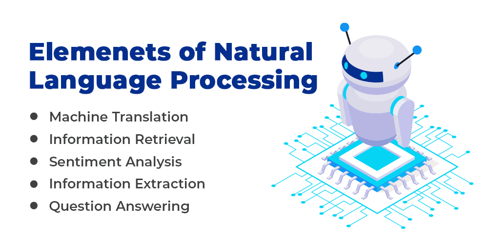
Every company wants to incorporate it in some way into its operation. We need to look at the applications of natural language processing to comprehend its potential and how it will affect our daily lives. Let’s begin with the applications of natural language processing in real life –
- Search Autocomplete and Correction – Every time you perform a search on Google, it suggests additional search terms after you type the first two or three letters. Or, if you type in a typo while searching, it will still find results pertinent to your search. Isn’t it incredible? Everyone uses it daily, but no one ever gives it much thought. It’s a beautiful example of how natural language processing is being used and how it affects people like you, me, and millions worldwide. Both searches, autocomplete and autocorrect, assist us in efficiently finding accurate results. Numerous other businesses, including Facebook and Quora, have begun utilizing this characteristic on their websites.
- Social Media Monitoring – Many people now use social media to express their opinions about various products, policies, and topics. These might have some helpful information regarding a person’s preferences. Consequently, by analyzing this unstructured data, valuable insights can be gained. Natural language processing also steps in to help. Today, businesses analyze social media posts to learn what their customers think of their products using various NLP technology. Additionally, firms use social media monitoring to learn about the issues and difficulties that their customers are having with their products. Even the government uses it to spot potential threats to national security, not just businesses.
- Voice Assistants – You have probably already met Google Assistant, Apple Siri, and Amazon Alexa. A voice assistant is software that interprets a user’s verbal commands and takes appropriate action using speech recognition, natural language understanding, and natural language processing. Most people today find it impossible to imagine life without voice assistants. They have evolved into a very dependable and robust friend. A voice assistant can do anything, such as setting our alarm for the morning or locating a restaurant. Both users have unlocked new doors of opportunity.
NLP case studies
- Roche – Roche is the top in-vitro diagnostics company in the world, and more than 130 million people are treated with its medications each year. To extract clinical information from pathology and radiology reports, Roche is using Spark NLP technology for Healthcare. Unstructured free-text data is the only source of many crucial facts needed by healthcare AI applications like patient risk prediction, cohort selection, and clinical decision support. The level of accuracy achieved for tasks like biomedical named entity recognition, assertion status detection, entity resolution, and de-identification has increased due to recent advances in deep learning. The first large-scale application of these new findings and its industrial-grade implementation is presented in this case study.
- Select Data – Many companies still rely on documents stored as images, including contracts, waivers, leases, forms, and audit records scanned from receipts, manifests, invoices, medical reports, and ID cards. There are three difficulties in extracting high-quality information from these images. The first is OCR, as in working with wrinkled receipts taken at an angle in a dark room. The second method is NLP, which pulls normalized values and entities out of text written in natural language. The third step entails creating predictors or recommendations that suggest the best course of action, especially when dealing with inaccurate or inconsistent data produced by the previous steps. In this case study, an AI system is shown to read millions of pages of patient data from various sources, producing a wide range of image formats, templates, and quality. The solution architecture is examined, along with the critical insights gained in the transition from raw images to a deployed predictive workflow based on information gleaned from the scanned documents.
- UiPath – Even for human domain experts, accurately responding to queries based on data from financial documents—which can be over a hundred pages long—is challenging. It is easier to infer facts based on implied statements, the absence of specific words, or the combination of other points than it is to do so using traditional rule-based or expression-matching techniques for simple fields in templated documents. Modern deep learning methods combined with NLP Big Data are required to answer such questions with a very high level of accuracy.
NLP Big Data
Natural Language Processing, which enables big data to extract information using cutting-edge techniques to produce valuable insights on current and projected market trends, is regarded as the next big thing in data analytics. The study of how computers and languages interact is called “natural language processing,” or NLP. NLP is a subfield of data science and artificial intelligence. NLP aims to program a computer to comprehend spoken human language.
NLP Use
Computer programs that translate text between languages respond to spoken commands, and quickly summarize large amounts of text—even in real-time—are all powered by NLP. However, the use of NLP in real life in enterprise solutions is expanding as a means of streamlining business operations, boosting worker productivity, and streamlining mission-critical business procedures. It is incredibly challenging to create software that accurately ascertains the intended meaning of text or voice data because human language is rife with ambiguities. Thus, NLP can help teachers enhance the quality of instruction within specific assignments and the learning environment as a whole. In addition to directly improving students’ language abilities, NLP features can also be used by teachers to comprehend better what is occurring cognitively with their students.
NLP and Data Science
Machine learning is the foundation of current approaches to NLP, which look for patterns in natural language data and use those patterns to enhance a computer program’s language comprehension. Chatbots, smartphone personal assistants, search engines, banking apps, translation software, and many other business applications use natural language processing technologies to parse and comprehend spoken and written human language. Extensive data integration is the critical element that makes all of that clever marketing, first-rate customer service, strategic upselling, etc., possible.
Text Processing The Language of Machines: The Evolution of Natural Language Processing
Text processing, in easy terms, refers to the manipulation and analysis of textual facts using computer algorithms. It includes various responsibilities inclusive of cleaning and organizing text, extracting significant facts, and reworking textual content records into a format that may be effortlessly understood and analyzed through machines. Text processing is a vital step in natural language processing (NLP) and helps computer systems recognize, interpret, and generate human language. It is broadly used in programs like sentiment analysis, language translation, chatbots, And record’s retrieval.
╔═════════════════╗
║ Text Processing – Why and Where ║
╚═════════════════╝
│
┌─────┴─────┐ [Tokenization]
│ Lowercasing │ Used for uniformity in text by converting all words to lowercase.
│ Stemming │ Reduces words to their root/base form to capture core meaning.
│ Lemmatization│ Similar to stemming but considers context, providing more accurate results.
└──────┬──────┘
│
┌─────┴─────┐ [Stopwords]
│Stopwords│ Removal of common words that carry little semantic meaning, improving analysis accuracy.
└─────┬─────┘
│
┌─────┴─────┐ [One Hot Encoding]
│ Encoding │ Converts text into numerical vectors, essential for machine learning models.
└─────┬─────┘
│
┌─────┴─────┐ [Word2Vec]
│ Word2Vec │ Represents words in vector space, capturing semantic relationships for better understanding.
└─────┬─────┘
│
┌─────┴─────┐ [Gensim]
│ Gensim │ Library for topic modeling and document similarity analysis.
└─────┬─────┘
│
┌──────┴──────┐ [Sentiment Analysis]
│ Sentiment │ Evaluates the emotion expressed in the text.
└──────┬──────┘
│
┌────┴─────┐ [Output]
│ Output │ Final processed text ready for analysis or further applications.
└─────────┘
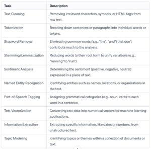
This table outlines key textual content processing tasks, starting from preliminary textual content cleansing and tokenization to superior obligations like sentiment evaluation and subject matter modeling. These processes are crucial for extracting significant insights from unstructured text records in fields including natural language processing and system getting to know.
Let’s talk about the dataset types.
What is Structured & Unstructured Data
They are dependent statistics, which possesses organized and smooth to keep in databases or tables facts.
Characteristics:
Tabulated layout; this data appears in a shape of rows and columns as that of unfold sheet /relations database.
Defined Schema; the information is established in a manner that only certain kinds and types of data kinds exist.
The reason for clean query inside the case of structured information is its orderly shape. Database question language which includes SQL may be used to query them.
Examples:
Database utilized by the ERP machine.
Excel spreadsheets.
The patron facts held in a CRM machine.
Financial records.
What is unstructured data and examples?
Unstructured records denote any facts without a pre-given shape or pattern. Nothing about it’s far organized at all. Hard to classify into traditional databases.
Characteristics:
No set shape; Unstructured statistics is not prepared at a given body that offers it adaptability however also may be challenging in some instances.
For instance, it may present itself below extraordinary formats, including textual content form, pix, video, audio files, and social media posts.
It is difficult to search for facts that can be extracted from facts through the use of complicated mechanisms including natural language processing or gadget mastering.
Examples:
The diverse styles of documents that incorporate this canister consist of phrase and pdf articles. Emails.
Social media updates.
Various types of media including pictures, audio, and films, Web pages.
There are also intermediates, such as partially structured data with parts of structured and unstructured data.
In this case, the partially structured data is partially structured although not as well structured as the fully structured data. For example, there are some guidelines that not everyone has to follow strictly. It’s a very simple format, which, usually, is expressed in formats like JSON or XML.
For example, it can be web data, such as on the web, or other hierarchical files that are not in a strict order.
– This data structure is usually nested hierarchically.
– Simple layouts can show more detailed information, such as home/work and other phone numbers.
– For example, when it comes to “interests”, they may be smaller than others.
– This refers to the semi-structured format of the data, with some structure (nested objects and arrays) and flexibility regarding content.
Today, one of the largest sources of information is unstructured and one of the most important sources of information in the modern world.
For example
– This involves seeking customer opinion from product reviews or reviews.
– Insights from social media data extracts.
Why do we use it?
– Extracting meaningful insights from unstructured textual data is not a “piece of cake”.
– Requires extensive data preprocessing.
Note:
– When the data is clean and ready, we use an algorithm (regression, classification, or clustering).
– One example is stock market price changes based on news.
– In this case, the attributes are associated with positive or negative attitudes towards a particular company.
– Uses text data segmentation to organize its positive and negative emotions based on the customer’s review information.
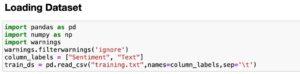
Let’s understand text processing by a python implementation.
What do you mean by dataset?
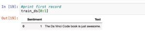
The data reflects the emotions applied to films.
Every statement listed here is a record, categorized as positive or negative.
The dataset includes:
Text: Actually, a review of the movie.
Emotions: Positive emotions are recorded as 1 and negative emotions as 0.
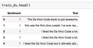
Inference about the data set
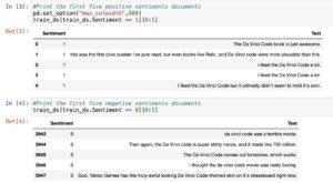
– Some text may be truncated when printing because the default column width is small.
– This can be changed by using the ‘max_colwidth’ parameter to increase the width size.
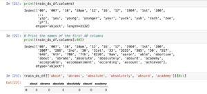
Document: Each record or example in the column text.
In herbal language processing (NLP), a “record” usually refers to a bit of text or a collection of textual content that is being analyzed or processed. A report can range in length and shape, starting from a brief sentence or paragraph to a whole e book. It is basically a unit of textual content that is taken into consideration as a single entity for evaluation.
What is the exploratory data analysis
In the context of Natural Language Processing (NLP), EDA typically stands for “Exploratory Data Analysis.” Exploratory Data Analysis is a vital step in information and gaining insights from a dataset before making use of machine getting to know or statistical models. While EDA is more usually associated with established statistics, inclusive of numerical and specific functions in tabular datasets, the principles can also be implemented to text records in NLP.
In NLP EDA, you would possibly carry out various analyses and visualizations to recognize the traits of the text information, such as:
Characteristic | Description
Token Distribution | Analysis of the distribution of words or tokens in the corpus.
Document Lengths | Examination of the distribution of document lengths.
Word Frequencies | Identification of the most and least frequent words in the corpus.
N-grams Analysis | Exploration of the distribution of n-grams for context understanding
Part-of-Speech
(POS) Tagging | Analysis of the distribution of different parts of speech.
Topic Modelling | Application of techniques to identify prevalent topics in the dataset
Sentiment Analysis | Investigation of sentiment label distribution in sentiment analysis.
EDA in NLP facilitates practitioners and researchers gain a deeper information of the language statistics they are running with, that is critical for making informed selections concerning preprocessing, feature engineering, and model selection.
For instance,
– We can check what number of opinions are to be had in the dataset?
– Are the high-quality and terrible sentiments evaluations well represented in the dataset?
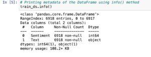
Inference:
– There are 6918 statistics to be had in the dataset.
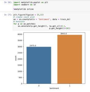
– We create a be counted plot to compare the number of fine and terrible sentiments.
This code is creating a depend plot the usage of the Seaborn library (sn). Here’s a breakdown of the code:
plt.Parent(figsize=(6,5)): This units the size of the figure (plot) to be created. The discern size is certain as a tuple (width, height). In this case, it is 6 devices wide and five devices tall.
Ax = sn.Countplot(x=’Sentiment’, facts=train_ds): This line uses Seaborn’s countplot characteristic to create a bar plot of the counts of every precise cost in the ‘Sentiment’ column of the train_ds DataFrame. The resulting plot is assigned to the variable ax.
The for p in ax.Patches loop iterates over every bar within the count number plot.
Ax.Annotate(p.Get_height(), (p.Get_x() zero.1, p.Get_height() 50)): For each bar, this line annotates the plot via adding text. It makes use of p.Get_height() to get the peak of the bar, and (p.Get_x() 0.1, p.Get_height() 50) specifies the coordinates in which the textual content annotation can be positioned. The 0.1 and 50 are used to adjust the position for better visibility.
In summary, this code generates a remember plot of sentiment values in the ‘Sentiment’ column of the train_ds DataFrame, and it provides annotations above every bar indicating the rely for that sentiment class. Adjustments are made to the placement of the annotations for better readability.
Inference: *
– There are general 6918 statistics in the dataset.
– Out of 6918 facts, 2975 information belongs to poor sentiments, whilst 3943 information belong to tremendous sentiments.
– Positive and terrible sentiment files have pretty same illustration inside the dataset.
What are the feature extraction techniques for textual data?
In the world of herbal language processing (NLP) and system gaining knowledge of, coping with unstructured text information offers a unique venture. Unlike established statistics with predefined capabilities, text information calls for a system to extract meaningful information. This is in which characteristic extraction turns into crucial.
Bag of Words (BoW) Approach:
The Bag of Words (BoW) approach is a essential technique to transform text records into a based format suitable for device studying algorithms. Here’s how it works:
Word as Features:
In BoW, every word within the text is handled as a distinct characteristic. The vocabulary is largely a collection of all unique phrases across the whole dataset.
Presence or Absence:
BoW specializes in the presence or absence of phrases in a report, disregarding the order or structure of the phrases. This simplification lets in for a mathematical representation of text.
Document as a “Bag”:
Each record (sentence or paragraph) is taken into consideration a “bag” containing a mix of words. The order of words is unnoticed, and handiest their occurrence topics.
Document, Sentence, and Corpus:
Document:
In the context of textual content analysis, a report refers to an character unit of text. This may be a sentence, a paragraph, or any coherent piece of facts.
Sentence as Document:
For the reason of BoW, each sentence is dealt with as a separate document. This desire enables the evaluation of person sentences in isolation.
Corpus:
The corpus represents the complete collection of files. It encompasses all of the sentences or paragraphs under consideration.
BoW Implementation:
Numerical Matrix: BoW transforms the textual content into a numerical matrix, where every row corresponds to a record, and each column corresponds to a unique phrase inside the vocabulary.
Binary Representation:
The entries inside the matrix are binary, indicating whether a particular word is present (1) or absent (0) in a particular file.
Significance:
BoW, at the same time as a simplistic representation, lays the inspiration for extra superior NLP strategies. It allows machines to “recognize” text by associating numerical values with words, paving the manner for the application of device studying fashions to unstructured textual facts.
Natural Language Processing: Bag-of-Words(BOW) Implementation
Step 1: Creating a BoW Model
In step one, we build a BoW model to create a dictionary of all the unique phrases used inside the corpus. This process entails:
Word Extraction:
Identify all awesome phrases throughout the whole corpus. Grammar and phrase order are unnoticed; handiest the incidence of phrases topics.
Dictionary Creation:
Form a dictionary in which every specific word is assigned a unique identifier or index. This dictionary encapsulates the whole vocabulary of the corpus.
Step 2: Convert Each Document to a Vector
In the second step, we convert each report (sentence or paragraph) into a vector that represents the presence or absence of phrases in that document. The steps consist of:
Document Tokenization:
Tokenize every report, breaking it down into person words.
Vector Representation:
Create a vector for each file, with dimensions corresponding to the words in the vocabulary. The values inside the vector imply whether or not a selected word is present (1) or absent (zero) within the record.
Significance of BoW:
Simplicity:
BoW simplifies complicated textual information right into a conceivable format for system studying models.
Numerical Representation:
Converts textual content into a numerical matrix, allowing mathematical operations.
Feature Extraction:
Facilitates the extraction of capabilities from textual content for downstream NLP obligations.
Versatility:
BoW serves as a foundational idea for numerous advanced NLP strategies and fashions.
BoW, although primary, lays the basis for greater sophisticated approaches, presenting a dependent representation of textual statistics for effective gadget getting to know analysis
Why Bow Words Are Important?
Bag of Words (BoW) serves as a essential approach in Natural Language Processing (NLP), contributing to various models for text evaluation. Here are three critical BoW-derived models:
- Count Vector Model:
Definition:
In this version, every record is represented as a vector where every element corresponds to the be counted of a specific phrase within the document.
Importance:
Captures the frequency of words, supplying a easy yet powerful illustration of report content material.
- Term Frequency Vector Model:
Definition:
Represents files as vectors, with each element indicating the frequency of a phrase inside the record divided by using the entire range of words in that document.
Importance:
Considers the relative significance of words, presenting a normalized measure that bills for various record lengths.
- Term Frequency-Inverse Document Frequency (TF-IDF) Model:
Definition:
Evaluates the significance of a word in a report relative to its prevalence across the whole corpus.
Importance:
Assigns better weights to phrases that are frequent in a record however uncommon in the whole corpus, emphasizing their importance.
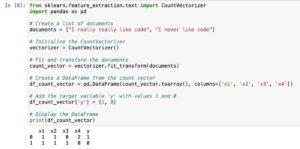
Count Vector Model Example:
Let’s explore the Count Vector Model the use of sample files, one with tremendous sentiment and any other with bad sentiment.
Document 1 (Positive Sentiment):
“The product is awesome, and the customer service is extremely good. I notably advocate it!”
Document 2 (Negative Sentiment):
“The quality of the product is negative, and the customer service is terrible. I would now not recommend it.”
Count Vector Representation:
We create a vocabulary based totally on all particular words inside the two files:
Vocabulary: the, product, is, exceptional, and, consumer, service, tremendous, I, rather, advise, it, high-quality, of, poor, horrible, might, no longer.
The Count Vector for each report represents the matter of each word from the vocabulary:
Document 1: [1, 1, 2, 1, 1, 1, 1, 1, 1, 1, 1, 1, 0, 0, 0, 0, 0, 0]
Document 2: [2, 1, 2, 0, 1, 1, 1, 0, 1, 0, 1, 1, 1, 1, 1, 1, 1, 1]
This illustration quantifies the frequency of each word inside the files, growing numerical vectors that can be used as capabilities for gadget studying fashions. The Count Vector Model simplifies complicated text information right into a format appropriate for analysis and modelling.
Inference:
The Count Vector Model serves as a fundamental approach in natural language processing for changing textual content facts right into a layout suitable for system getting to know models. Here’s a extra certain breakdown:
Vocabulary Set Creation:
The procedure starts offevolved with the introduction of a vocabulary set that includes all particular words present inside the given files. In our example, phrases like “I,” “certainly,” “in no way,” “like,” and “code” form this set.
Feature Representation:
Each word in the vocabulary set turns into a function, contributing to the creation of feature vectors. For instance, if the vocabulary set has N words, each document is represented as an N-dimensional vector.
Count Vectors:
The middle of the Count Vector Model entails counting the occurrences of every phrase in a document. This outcomes in a numeric illustration wherein each detail in the vector corresponds to the frequency of a selected phrase in the document.
Sentiment Representation:
The sentiment of every file is denoted in the y-column. For binary sentiment evaluation (superb or poor), 1 can symbolize fine sentiment, and 0 can represent negative sentiment.
Machine Learning Input:
The generated count vectors function input features for machine getting to know algorithms. These algorithms research styles and relationships between phrase frequencies and sentiments, permitting the model to predict sentiment for new, unseen textual content.
In precis, the Count Vector Model helps the transformation of uncooked textual content records right into a structured format, allowing machine getting to know fashions to extract significant insights and make predictions primarily based at the frequency of words in files.
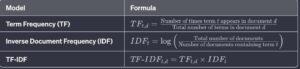
TF-IDF (Term Frequency – Inverse Document Frequency):
TF-IDF combines the ideas of TF and IDF to gauge the significance of a word in a selected file relative to its prevalence within the whole corpus. The calculation includes multiplying the TF cost (neighborhood importance) by means of the IDF fee (worldwide importance).
TF (Term Frequency):
TF for a term in a file is calculated because the frequency of that time period in the document divided through the overall wide variety of terms within the document.
IDF (Inverse Document Frequency):
IDF for a term is calculated as the logarithm of the entire number of documents divided by means of the quantity of files containing the term.
Importance Assessment:
TF: Reflects how often a term seems within a selected report.
IDF: Indicates how unique or rare a term is throughout the entire corpus.
TF-IDF: Measures the importance of a time period within a report while considering its rarity across the corpus.
Visualization: Python Implementation
The IDF values for the phrases within the furnished documents are displayed within the accompanying picture, showcasing the varying significance of each time period based on their occurrences inside the corpus.
In precis, the TF Vector Model, IDF, and TF-IDF together offer a nuanced knowledge of time period importance, allowing more sophisticated analyses and machine gaining knowledge of packages in herbal language processing.
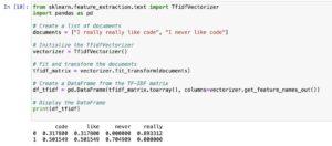
Python implementation,
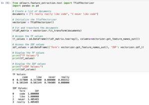
This code snippet demonstrates the usage of TfidfVectorizer from scikit-discover ways to calculate TF (Term Frequency) and IDF (Inverse Document Frequency) values for a set of documents. Here’s a step-by way of-step explanation:
Import Libraries:
from sklearn.Feature_extraction.Textual content import TfidfVectorizer
import pandas as pd
Create Documents:
documents = [“I really really like code”, “I never like code”]
This is a list of two files.
Initialize TfidfVectorizer:
vectorizer = TfidfVectorizer()
Initialize the TfidfVectorizer, a good way to help in remodeling the textual content facts into TF-IDF functions.
Fit and Transform Documents:
tfidf_matrix = vectorizer.Fit_transform(files)
Fit and remodel the files the use of TfidfVectorizer. This step calculates both TF and IDF values.
Access TF Values:
tf_values = pd.DataFrame(tfidf_matrix.Toarray(), columns=vectorizer.Get_feature_names_out())
Create a DataFrame to show the TF values for every term inside the files.
Access IDF Values:
idf_values = pd.DataFrame(‘Term’: vectorizer.Get_feature_names_out(), ‘IDF’: vectorizer.Idf_)
Create a DataFrame to display the IDF values for every term.
Display Results:
print(“TF Values:”)
print(tf_values)
print(“nIDF Values:”)
print(idf_values)
Print the TF and IDF values.
In precis, the code utilizes TfidfVectorizer to transform the text statistics into TF-IDF representation and then extracts and shows the TF and IDF values in tabular form.
The TF-IDF values for the two documents.
Sparse Matrix:
In simple phrases, a sparse matrix is a form of matrix where maximum of the elements are 0. Instead of storing all of the elements in a ordinary or dense matrix, a sparse matrix most effective stores the non-0 factors and their positions.
Example:
Consider a matrix representing the relationships between college students and the publications they’ve taken. Most students take only a few guides, leading to a matrix with ordinarily 0 values.
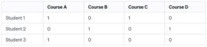
In this sparse matrix example:
Instead of storing all entries, we simplest keep the non-zero values (1s in this case).
We also keep the positions of these non-0 values, indicating which scholar took which path.
Sparse matrices are useful in saving reminiscence and computational resources whilst handling massive datasets with many 0 values, as we handiest consciousness at the non-0 factors.
One-hot coding, Word2Vec, and averaging Word2Vec are all strategies used for representing words in a numerical layout in herbal language processing (NLP). Let’s wreck down each of them:
Text Encoding in Natural Language Processing (NLP) & Types
One-warm encoding is a technique used to symbolize categorical variables, such as phrases within the context of natural language processing (NLP). There are diverse methods to carry out one-hot encoding relying on the unique necessities. Here are a few varieties of one-warm encoding:
Simple One-Hot Encoding:
In this technique, each precise phrase is assigned a unique index, and a binary vector is created with all zeros besides for the index corresponding to the word, which is set to at least one.
Example:
from sklearn.Preprocessing import OneHotEncoder
import pandas as pd
Sample data
statistics = ‘Words’: [‘apple’, ‘orange’, ‘banana’, ‘apple’, ‘banana’]
df = pd.DataFrame(data)
Initialize OneHotEncoder
encoder = OneHotEncoder(sparse=False)
pply one-hot encoding to the ‘Words’ column
one_hot_encoded = encoder.Fit_transform(df[[‘Words’]])
print(one_hot_encoded)
Binary One-Hot Encoding:
Similar to easy one-warm encoding, however the binary vector is represented as zero and 1 instead of indices.
Example:
# Using pandas get_dummies
one_hot_encoded_binary = pd.Get_dummies(df[‘Words’])
print(one_hot_encoded_binary)
Customized One-Hot Encoding:
In a few cases, you would possibly need to customize the encoding based on precise standards, which includes phrase frequency or relevance.
Example:
from sklearn.Feature_extraction.Textual content import CountVectorizer
# Using CountVectorizer for custom one-hot encoding
vectorizer = CountVectorizer(binary=True)
custom_one_hot_encoded = vectorizer.Fit_transform(df[‘Words’])
print(custom_one_hot_encoded.Toarray())
Multi-Hot Encoding:
Allows for a couple of occurrences of a word inside a report, resulting in a binary vector with multiple 1s for repeated occurrences.
# Using CountVectorizer for multi-hot encoding
vectorizer_multi_hot = CountVectorizer(binary=True)
multi_hot_encoded = vectorizer_multi_hot.fit_transform(df[‘Words’].apply(lambda x: ‘ ‘.join(x)))
print(multi_hot_encoded.toarray())
Choose the method that best fits your specific NLP task and data characteristics.
Word2Vec:
Word2Vec is a popular phrase embedding approach that represents phrases in dense vectors of continuous values. It captures the semantic relationships between phrases and is skilled the use of neural networks. Word2Vec typically affords better phrase representations as compared to one-hot coding.
Averaging Word2Vec:
Averaging Word2Vec is a simple technique where the vector illustration of a document is obtained by averaging the Word2Vec vectors of all the words in that report. It’s a brief and powerful manner to symbolize a record as a non-stop vector.
from gensim.models import Word2Vec
from gensim.models import KeyedVectors
import numpy as np
# Example sentences
sentences = [[“I”, “really”, “like”, “code”], [“I”, “never”, “like”, “code”]]
# Train Word2Vec model
model = Word2Vec(sentences, vector_size=100, window=5, min_count=1, workers=4)
word_vectors = model.wv
# Function to average Word2Vec vectors
def average_word_vectors(words, model, vocabulary, num_features):
feature_vector = np.zeros((num_features,), dtype=”float64″)
n_words = 0
for word in words:
if word in vocabulary:
n_words += 1
feature_vector = np.add(feature_vector, model[word])
if n_words:
feature_vector = np.divide(feature_vector, n_words)
return feature_vector
# Vocabulary
vocabulary = set(model.wv.index_to_key)
# Averaging Word2Vec for each sentence
avg_vectors = [average_word_vectors(sentence, model, vocabulary, 100) for sentence in sentences]
# Display the averaged vectors
print(“Averaged Word2Vec Vectors:”)
print(avg_vectors)
This code demonstrates a way to use the Word2Vec model from the gensim library to train word embeddings on a small set of instance sentences after which calculate the common word vectors for each sentence.
Here’s an explanation of the code:
Import Libraries and Load Sentences:
Import necessary libraries: Word2Vec from gensim.Models, KeyedVectors, and numpy.
Define example sentences.
Train Word2Vec Model:
Train a Word2Vec version using the supplied sentences.
Parameters:
vector_size: Dimensionality of the word vectors (set to a hundred in this situation).
Window: Maximum distance among the cutting-edge and expected word inside a sentence.
Min_count: Ignores all phrases with a total frequency decrease than this.
Employees: Number of CPU cores to apply for education.
Define Averaging Function:
Define a function (average_word_vectors) to calculate the average word vectors for a listing of phrases the usage of the trained Word2Vec version.
It initializes a characteristic vector with zeros and iterates thru the phrases, including the vectors of every phrase in the vocabulary.
Create Vocabulary:
Extract the vocabulary from the trained Word2Vec version.
Averaging Word Vectors for Sentences:
Calculate the common Word2Vec vectors for each sentence using the defined characteristic.
Display the averaged vectors.
Note: The Word2Vec model is skilled on a completely small dataset in this case. In exercise, you will use a extra large dataset for significant phrase embeddings. The averaged vectors can be used as features for numerous NLP obligations.
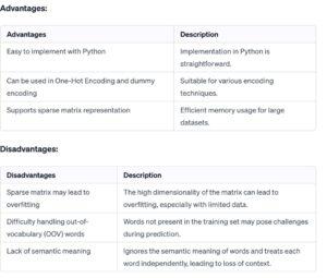
Let’s summarize the advantages and disadvantages of using the Bag of Words (BoW) model in a table:
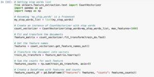
Creating Count Vectors for sentiment_train Dataset
In herbal language processing (NLP), remodeling text statistics into numerical vectors is essential for device learning models. One popular technique is the Bag of Words (BoW) model, which represents every file as a vector of phrase frequencies
CountVectorizer in sklearn.Feature_extraction.Text
The CountVectorizer is a feature extraction method normally utilized in Natural Language Processing (NLP) to convert a set of text files right into a matrix of token counts.
Initialization:
It is part of the sklearn.Feature_extraction.Text module in Python.
Creating Count Vectors:
How it Works:
Treats each document as a “bag of words” idea.
Builds a vocabulary from all particular words in the corpus.
Represents every file as a vector, in which each detail denotes the rely of a selected word.
Example Scenario:
For example, given two files “I truely like code” and “I by no means like code,” the resulting remember vectors could mirror the word frequencies for every report.
Resulting Sparse Matrix:

The output is a sparse matrix wherein rows represent files, and columns represent unique words.
The matrix is sparse due to the fact maximum documents may not incorporate every word from the vocabulary.
Accessing Features:
After transformation, access the depend vectors and characteristic names for further evaluation.
Usage in Machine Learning:
Count vectors generated by way of CountVectorizer function input capabilities for machine getting to know models.
Particularly useful for duties like text classification, sentiment evaluation, and different NLP programs.
In essence, CountVectorizer helps the conversion of text information into a established numerical layout appropriate for machine mastering algorithms, shooting the incidence of every word throughout distinct documents for evaluation and version training.
CountVectorizer Operation Explanation: Vectorization Techniques in NLP:
How it works?
Building a Dictionary:
Input: Documents
The CountVectorizer starts offevolved through growing a dictionary that contains all precise phrases observed throughout all documents inside the corpus.
Feature Representation:
Dictionary Entries as Features:
Each particular word inside the dictionary becomes a feature. These functions will be used to symbolize the documents.
Counting Occurrences:
Count Vector Creation:
For each document, the CountVectorizer counts the occurrences of every word (feature) in that report.
Sparse Matrix Formation:
Document-Word Matrix:
The end result is a matrix where rows constitute files, and columns represent specific words (capabilities).
Sparse Matrix Properties:
Sparsity:
Due to the nature of language, in which a small set of phrases is utilized in each record, the ensuing matrix is often sparse (in general zeros).
Output:
Sparse Matrix Output:
The output is a sparse matrix that successfully represents the frequency of each phrase across the complete set of files.
Ready for ML Models:
Input for Machine Learning:
This sparse matrix is then used as enter capabilities for gadget gaining knowledge of fashions, allowing algorithms to examine styles primarily based on word occurrences.
CountVectorizer hence transforms uncooked textual content facts right into a based numerical format, laying the foundation for diverse herbal language processing responsibilities with the aid of representing documents as depend vectors based on the frequency of words in the corpus.
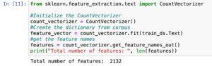
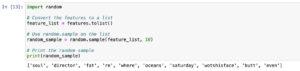
Random Sampling Features:
Total Features:
The corpus consists of a total of 2132 particular words, each taken into consideration as a function.
Random Sampling:
random.Pattern():
The code snippet makes use of the random.Pattern() technique to reap a random sample of functions from the entire set.
Purpose of Sampling:
Subset for Display:
The random sampling is probable used for display purposes or to analyze a practicable subset of capabilities as opposed to the whole set.
Application:
Visualization or Analysis:
This sampling method will be implemented whilst exploring or visualizing the capabilities to gain insights into the characteristics of the words in the corpus.
Iterative Sampling:
Repeatable Process:
If necessary, the sampling technique can be repeated, ensuring a distinctive set of random functions for every generation.
Maintaining Diversity:
Randomness for Diversity:
The use of randomness helps hold range inside the sampled capabilities, imparting a consultant subset of the whole function space.
Sampling capabilities offers a glimpse into the variety of phrases present inside the corpus and aids in expertise the composition of the vocabulary used across documents.
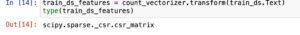
How to convert a text document to a vector? Steo by Step Process
Feature Dictionary:
The dictionary, created from all words in the corpus, serves as the function set.
Transformation Process:
The transform() technique of the CountVectorizer is employed to convert files into remember vectors.
Count Vector Representation:
Each file’s illustration includes the count of occurrences for each phrase (characteristic) in the dictionary.
Vectorization Purpose:
This technique is essential for turning uncooked textual content right into a format suitable for machine getting to know fashions that require numerical input.
Numerical Encoding:
Words are encoded numerically, permitting algorithms to procedure and examine textual facts correctly.
Document-to-Vector Mapping:
Documents are mapped to vectors, facilitating the extraction of features and patterns inside the dataset.
Machine Learning Compatibility:
The ensuing count vectors emerge as the input features for device learning fashions.
Data Transformation:
Count vectorization transforms the text statistics right into a dependent and numerical format, permitting the application of various algorithms.
Converting files to be counted vectors is an essential step in getting ready textual content facts for system studying tasks, permitting the utilization of powerful algorithms for evaluation and prediction.
Understanding Dimensions of Count Vectors DataFrame:
DataFrame Overview:
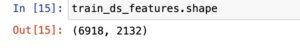
The DataFrame train_ds_features holds the count number vectors of all documents within the sentiment_train dataset.
Shape Attribute:
The shape of the DataFrame, handy via the shape attribute, offers records approximately its dimensions.
Dimensions Interpretation:
The dimensions are represented as (rows, columns), in which rows correspond to the number of files, and columns indicate the quantity of capabilities (specific words).
Example:
If the shape is (5000, 2132), there are 5000 documents (rows) and 2132 features (columns) within the DataFrame.
Document Count:
The range of rows indicates the whole count number of files within the dataset.
Feature Count:
The wide variety of columns represents the matter of unique phrases or features in the whole corpus.
Understanding the dimensions of the DataFrame is essential for comprehending the shape and scale of the depend vectors, aiding in subsequent analysis and model building techniques.
Understanding Sparse Matrix and its Representations:
Sparse Matrix Overview:
After vectorizing files, the end result is a sparse matrix with 2132 features.
Dimensional Insights:
Each file is represented by a matter vector of 2132 dimensions, reflecting the remember of particular words.
Sparse Matrix Definition:
Due to documents containing few phrases, many dimensions in vectors have values set to zero, ensuing in a sparse matrix.
Optimization with Sparse Matrix:
Sparse matrix illustration stores handiest non-zero values and their indices, optimizing storage and computational performance.
Dealing with zero’s:
Since most dimensions have zero values, a sparse matrix correctly handles the abundance of zero’s inside the matrix.
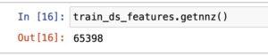
Getnnz() Method:
The getnnz() method at the DataFrame famous the be counted of real non-0 values inside the matrix.
Understanding the sparse matrix representation aids in managing reminiscence utilization, hastens computation, and is in particular beneficial for datasets with severa zero values within the vectors.
The share of non-0 values to zero values within the matrix may be calculated by using dividing the wide variety of non-zero values (65398) by means of the whole range of elements inside the matrix (6918 * 2132), which leads to 65398 / (6918 * 2132). This computation presents perception into the sparsity of the matrix and facilitates understand the density of actual records inside the records representation. In this situation, it quantifies how lots of the matrix is populated with non-0 values in comparison to the full possible entries.
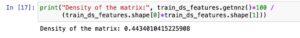
- The sparse matrix representation is utilized when many entries in a matrix are 0.
- In this situation, much less than 1% of the matrix values are non-0, indicating a excessive degree of sparsity.
- Sparse matrices shop handiest non-0 values and their corresponding indices, optimizing garage and computational performance.
- This approach is mainly beneficial in excessive-dimensional datasets in which many capabilities have zero occurrences in the files.
- The sparse illustration is completed via techniques just like the getnnz() technique, offering insights into the share of non-0 values relative to the matrix dimensions.
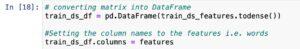
Displaying document vectors:
- The remember vectors, represented as a sparse matrix, can be visualized by changing them right into a DataFrame.
- The column names of the DataFrame are set to the actual characteristic names, providing a clean representation of the file vectors.
- This step aids in information the occurrence of each word across the documents and their respective counts.
- DataFrame visualization enables smooth interpretation of the record vectors, contributing to powerful exploratory facts evaluation (EDA) in herbal language processing (NLP).
- Due to the excessive dimensionality of the matter vectors (2132 dimensions), it is impractical to print the entire vector.
- However, we can inspect specific dimensions to understand the encoding. For example, inspecting dimensions from index one hundred fifty to 157 allows us to take a look at the illustration of the phrase “awesome.”
- In this range, if the phrase “wonderful” is found in a file, the corresponding dimension can have a non-zero price, reflecting its remember inside the file.
- This partial inspection offers perception into the encoding of specific words inside the file vectors.

- In the depend on vector for the word “awesome,” the corresponding characteristic is set to 1, indicating its presence in the report. Meanwhile, the other functions stay 0.
- By choosing columns based totally at the words in a sentence, we will observe how each phrase is encoded inside the remember vectors. This permits us to apprehend the illustration of more than one words inside the vectors.
Yes, the feature in the count vector is appropriately set to 0.
Removing Low-frequency Words
One technique to deal with this problem is to eliminate low-frequency words.
Low-frequency phrases are words that arise very hardly ever in the corpus, and that they might not make contributions lots to the general meaning of the files.
By removing these low-frequency phrases, we can lessen the dimensionality of the characteristic area and attention on extra significant and relevant phrases.
Steps to Remove Low-frequency Words:
Count the Frequency of Each Word: Calculate the frequency of every word within the corpus.
Set a Threshold: Decide on a threshold frequency underneath which phrases might be considered low frequency.
Remove Low-frequency Words: Remove phrases that have a frequency underneath the set threshold.
Benefits of Removing Low-frequency Words:
Reduced Dimensionality: Removing low-frequency phrases reduces the wide variety of features, making the version greater plausible.
Focus on Important Words: By removing much less informative words, the model can attention on greater relevant and significant phrases.
Improved Generalization: The version may additionally generalize better to new, unseen statistics by way of averting overfitting to uncommon phrases.
Challenges:
Choosing the Threshold: Selecting the correct threshold involves a exchange-off. Too excessive a threshold might put off crucial phrases, at the same time as too low a threshold might not provide full-size dimensionality reduction.
By summing the columns of the count vector matrix, we can acquire the total occurrence of every characteristic or word in the entire corpus.
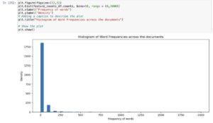
These facts may be used to create a histogram that suggests the distribution of word frequencies.
![]()
The histogram well-known shows that the distribution of phrase frequencies is exceedingly skewed to the right.
Most phrases have low frequencies, and simplest a small range of phrases arise regularly throughout files.
This is a common characteristic of natural language, where a small set of words (stopwords) appears frequently, at the same time as most words are used on occasion.
Handling Low-Frequency Words:
It is common to put off or clear out low-frequency words to reduce the dimensionality of the function space.
A threshold may be set, and words that occur much less often than the brink are eliminated.
This helps in focusing on the extra significant and informative words.
- Filtering functions with a count number same to 1 is one way to identify rare phrases within the dictionary.
- These words arise best in a single file inside the complete corpus.
- Removing such uncommon words may be useful as they will now not make contributions tons to the general know-how or class of files.
![]()
There are 1228 words which are present only once across all the documents in the corpus.
These words can be ignored.
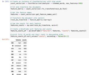
We can restrict the number of features by setting *max_features* parameters to 1000 while creating the count vectors.
- Setting the max_features parameter is a realistic approach to restriction the variety of features in the be counted vectors.
- By doing so, you most effective bear in mind the top N capabilities primarily based on their frequency within the corpus.
- This can be beneficial in lowering the dimensionality of the characteristic area and improving computational performance.
- Here’s how you could set max_features while growing count vectors:

- Adjust the price of max_features primarily based for your unique necessities and the characteristics of your dataset.
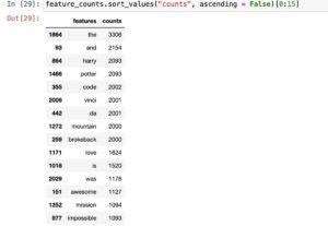
- It can be noticed that selected list of features contains words like **the, is , was, and* etc.
- These words area irrelevant in determining the sentiment of the document.
- These words are called stop words.
- It can be removed from the dictionary.
- This will reduce the number of features further.
Removing stop words
Stop words are normally used words that don’t contribute much to the overall meaning of a report.
Examples include articles (the, a, an), conjunctions (and, but), and not unusual prepositions (in, on, at).
Removing stop words is a common step in text preprocessing as they frequently do no longer carry much sentiment or content material-unique facts.
The stop_words parameter within the CountVectorizer may be used to exclude these phrases from the feature set.
Removing stop phrases can cause a extra focused and meaningful set of capabilities for sentiment evaluation. Adjust the parameters primarily based to your unique needs.
The stop_words parameter in CountVectorizer can be set to ‘english’ to apply a pre-described listing of English forestall words furnished by using scikit-learn.
This enables in doing away with not unusual English phrases that are frequently considered irrelevant in sentiment evaluation. Adjustments can be made based on unique necessities or languages.
Additional forestall phrases can be added to the prevailing listing the use of the stop_words parameter.
This allows for greater customization via which include area-precise or context-precise stop phrases that might not be present within the default list.
![]()
In Natural Language Processing (NLP), developing rely on vectors is a vital step to represent textual statistics in a layout appropriate for device mastering algorithms. Here’s the way it works:
Text Data: Begin with a set of files or sentences that you need to research. Each record is treated as a unit for analysis.
Tokenization: Break down every document into individual phrases or tokens. This method is called tokenization. For instance, the sentence “The meals is ideal” might be tokenized into [“The”, “food”, “is”, “good”].
Building a Vocabulary: Create a vocabulary, that’s a completely unique set of all phrases present inside the entire corpus (series of documents). Each word becomes a characteristic, and the vocabulary incorporates all viable capabilities.
Count Vectors: Convert each file into a vector that represents the frequency of every phrase in the document. The duration of the vector is equal to the dimensions of the vocabulary, and each detail within the vector corresponds to the matter of the respective phrase in the file.
Sparse Matrix: Represent the matter vectors in a sparse matrix. Since most files simplest include a subset of the whole vocabulary, the matrix is sparse, that means that many entries are 0. This illustration is reminiscence green.
Stop Words Removal: Optionally, cast off common prevent phrases (e.G., “the”, “is”, “and”) and rare phrases to reduce noise and enhance efficiency.
Analysis and Visualization: Analyse the ensuing be counted vectors to apprehend the distribution of words and their frequencies. Visualize the vectors to advantage insights into the shape of the textual content statistics.
By developing be counted vectors, text statistics is converted into a layout suitable for diverse machine gaining knowledge of algorithms, taking into consideration the extraction of significant styles and insights from textual.
Note:
- It’s obtrusive that the elimination of prevent phrases has been a success.
- However, any other task arises from the lifestyles of phrases in special forms, inclusive of “love” and “cherished.”
- The vectorizer treats those versions as wonderful words, main to redundancy.
- To address this, techniques like Stemming and Lemmatization come into play, aiming to reduce phrases to their root bureaucracy for greater meaningful evaluation.
Stemming
Stemming is a technique that aims to reduce phrases to their root forms with the aid of removing inflections or suffixes.
It includes slicing off the ends of phrases, probably ensuing in non-dictionary phrases.
For example, both “love” and “cherished” might be stemmed to the basis phrase “love.”
However, this procedure may lead to non-meaningful forms like “awesom” for each “extraordinary” and “awesomeness.”
Two famous stemming algorithms, PorterStemmer and LancasterStemmer, follow unique guidelines for word reduction.
Lemmatization
Lemmatization is a extra state-of-the-art approach as compared to stemming, as it reduces phrases to their base or dictionary shape.
Unlike stemming, lemmatization guarantees that the resulting phrases are meaningful and legitimate.
For example, both “love” and “loved” would be lemmatized to the base shape “love.”
Lemmatization entails searching up words in a lexicon or a vocabulary to find their base forms.
While stemming can cause non-dictionary phrases, lemmatization produces valid words with actual meanings.
In herbal language processing, lemmatization is regularly considered greater accurate, specifically when keeping phrase semantics is critical.
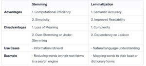
What are the Advantages and Disadvantages of Stemming and Lemmatization
Advantages:
Stemming:
Computational Efficiency: Stemming is computationally less high-priced compared to lemmatization, making it faster for massive datasets.
Simplicity: Stemming is a easier technique, and its rules are simpler to implement.
Lemmatization:
Semantic Accuracy: Lemmatization offers greater semantically correct outcomes because it maps words to their base or dictionary bureaucracy.
Improved Readability: The output of lemmatization includes valid phrases, which complements the interpretability and readability of the text.
Disadvantages:
Stemming:
Loss of Meaning: Stemming may additionally result in the lack of meaning, because it frequently produces root paperwork that aren’t actual phrases.
Over-Stemming or Under-Stemming: Depending at the rules, stemming algorithms may over-stem (reduce too much) or under-stem (go away an excessive amount of).
Lemmatization:
Complexity: Lemmatization is computationally extra complicated than stemming, and the system may be slower.
Dependency on Lexicon: Lemmatization is predicated on language dictionaries or lexicons, which won’t cover all possible phrases.
In practice, the selection among stemming and lemmatization depends on the particular necessities of the undertaking. Stemming may be preferred for performance in statistics retrieval or search engines like google and yahoo, while lemmatization is suitable while keeping the semantic accuracy of words is crucial, such as in natural language information packages.
What is Natural Language Toolkit (NLTK)
The Natural Language Toolkit (NLTK) is a extensively-used Python library for natural language processing (NLP) that gives various gear and sources for working with human language data. Here are some key features of NLTK:
Tokenization: NLTK provides methods for breaking text into words or sentences, making it less complicated to investigate and manner textual records.
Stemming and Lemmatization: NLTK helps exclusive stemming algorithms like PorterStemmer and LancasterStemmer, as well as lemmatization the use of WordNetLemmatizer. These strategies help reduce phrases to their root bureaucracy.
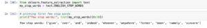
Stopwords: NLTK includes a listing of commonplace prevent words in English, which can be beneficial for filtering out beside the point words from textual content data.
Part-of-Speech Tagging: NLTK can assign elements of speech (e.G., noun, verb, adjective) to phrases in a sentence, aiding in syntactic evaluation.
Named Entity Recognition: NLTK presents gear for figuring out named entities (e.G., names of people, groups) in text.
Frequency Distributions: NLTK permits the evaluation of word frequencies, helping to pick out not unusual or uncommon words in a corpus.
Corpora and Resources: NLTK consists of diverse corpora and lexical sources for extraordinary languages, making it a precious tool for linguistic research.
Language Processing Pipelines: NLTK permits the advent of complete language processing pipelines, combining multiple NLP duties for greater superior analysis.
NLTK’s versatility and complete capability make it a favored choice for lots of researchers, developers, and statistics scientists running on NLP projects in Python.
When the use of CountVectorizer alongside NLTK for herbal language processing, you could create a application approach that consists of tokenization, stemming, and prevent word removal.
Here’s a high-degree instance the use of NLTK’s functionalities:
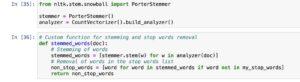
When making use of CountVectorizer with a custom analyzer for stemming and forestall phrase removal, you could define a custom feature, which includes stemmed_words. This feature performs tokenization, stemming, and gets rid of prevent phrases from the input text. The CountVectorizer is then initialized with this practice analyzer function, allowing the creation of rely vectors based totally on the processed phrases. This method helps in capturing essential functions whilst discarding not unusual prevent phrases and variations of words thru stemming, contributing to extra meaningful text representations. Adjustments may be made to the custom characteristic based totally on unique requirements or options.
It can be noticed that words *love, loved, awesome* have all been stemmed to the root words.
Through the stemming system, variations of phrases consisting of “love,” “cherished,” and “exceptional” had been converted into their root bureaucracy, enhancing consistency and reducing redundancy inside the text illustration. This is treasured for taking pictures in the centre which means of words and simplifying the function set inside the next analysis.
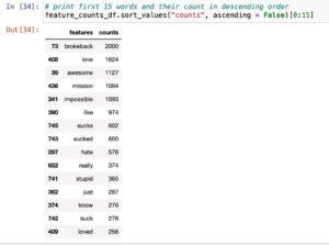
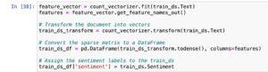
Distribution of Words Across Different Sentiment
Exploring the distribution of phrases across one-of-a-kind sentiments presents valuable insights into capability functions for sentiment evaluation. By studying how words with advantageous or poor connotations seem in documents of varying sentiments, we can perceive key signs that contribute to the overall sentiment of the textual content. This exploration lays the muse for deciding on applicable features that may drastically impact the accuracy of sentiment prediction fashions.
Consider the word ‘awesome’.
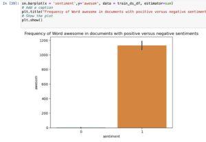
- As shown in figure, the word *awesom(stemmed word from awesome)* appears mostly in positive sentiment documents.
- How about a neutal word like *realli*?
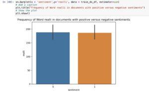
As shown, the word *realli(stemmed word for really)* occurs almost equally across positive and negative sentiments.
How about the word *hate*?
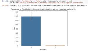
As shown, the word *hate* occurs mostly in negative sentiments than positive sentiments.
This absolutely make sense.
This gives us an initial idea that the words *awesom* and *hate* could be good features in determining sentiments of the document.
Naive bayes classifier explained for Sentiment Classification
Building a Naive-Bayes model for sentiment type entails leveraging the broadly followed Naive-Bayes classifier, an effective device in Natural Language Processing (NLP). This version operates on the foundational ideas of Bayes’ theorem, a statistical technique that calculates the chance of an occasion primarily based on earlier know-how of conditions that is probably related to that event.
In the context of sentiment evaluation, the Naive-Bayes classifier assumes that the capabilities (words in our case) are conditionally impartial, given the sentiment label. This assumption simplifies the calculations and makes the version computationally green, especially for big datasets. The version calculates the chance of a report belonging to a specific sentiment magnificence based on the prevalence of phrases in that document.
Despite its simplicity and the “naive” assumption of independence, Naive-Bayes classifiers often perform nicely in sentiment evaluation duties, making them a popular choice for text category.
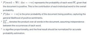
- Assume that we would like to predict whether the probability of a document is positive(or negative) given that the document contains a word awesome.
- This can be computed if the probability of the word awesome apperaring in a document given that it is a positive(or negative) sentiment multiplied by the probability of the document being positive(or negative).
P(doc = +ve| word = awesome) ∝ P(word = awesome | doc = +ve) * P(doc = +ve)
Allows destroy down the components of the expression:
- P (doc = +ve | word = awesome): This is the probability that a document is positive given that it contains the word “awesome.” It’s what we want to calculate.
- P (word = awesome | doc = +ve)P(word = awesome | doc = +ve): This is the probability of the word “awesome” appearing in a positive document. It represents how likely the word is associated with positive sentiments.
- p (doc = +ve)P(doc = +ve): This is the overall probability that a document is positive. It captures the general distribution of positive sentiments in the dataset.
The expression can be understood as follows:
- P (word = awesome | doc = +ve)P(word = awesome | doc = +ve): This term assesses how indicative the presence of the word “awesome” is for a positive sentiment. If “awesome” frequently appears in positive documents, this probability would be relatively high.
- p (doc = +ve)P(doc = +ve): This term reflects the general likelihood of a document being positive. It considers the proportion of positive documents in the entire dataset.
By multiplying those two chances, we gain an estimate of the probability that a report is wonderful given the presence of the word “terrific.” This is a fundamental idea in Bayesian statistics, in which we update our ideals (chance of high-quality sentiment) based totally on new evidence (presence of the word “extraordinary”). The proportional sign (∝) indicates that we’re working with proportional probabilities, and the very last result must be normalized to sum to 1 over all possible sentiment training.
The posterior probability of the sentiment is computed from the **prior** probabilities of all the words it contains.
The assumption is that the occurences of the words in a document are considered independent and they do not influence each other.
So, if the document contains N words and words are represented as W1, W2, ……WN, then

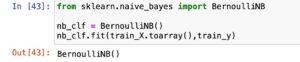
The Bernoulli Naive-Bayes (BernoulliNB) classifier in scikit-research is especially designed for scenarios in which functions are binary or Boolean, that means they may be both present and absent in each sample.
In the context of sentiment analysis or textual content type:
Binary Features: Each word in a record may be dealt with as a binary characteristic, in which the presence of the phrase is represented as 1, and its absence is represented as 0.
Multivariate Bernoulli Model: The time period “multivariate Bernoulli model” refers to the assumption that every characteristic (word) is binary and follows a Bernoulli distribution. In other phrases, the classifier assumes that the presence or absence of each word is independently and identically dispensed (i.I.D.).
Binary Classification: Since sentiment analysis frequently entails binary classification (wonderful or negative sentiment), the BernoulliNB classifier is nicely applicable for this assignment.
The BernoulliNB classifier calculates chances based totally at the presence or absence of phrases in files, making it appropriate for textual content classification troubles wherein the point of interest is at the prevalence of unique features rather than their frequency.
In precis, BernoulliNB is a preference while handling binary features, making it relevant to obligations like sentiment analysis, unsolicited mail detection, or another type of trouble regarding the presence or absence of functions.
Steps for sentiment analysis are as follow using Naive – Bayes:
Here’s a more distinct clarification of the steps for sentiment evaluation the usage of Naive-Bayes:
Split Dataset into Train and Validation Sets:
Purpose: The dataset is generally divided into subsets: one for training the model and the opposite for validating its performance.
Explanation: The education set is used to train the model the connection among functions (phrases in this situation) and their corresponding sentiments. The validation set is then used to evaluate how nicely the version generalizes to new, unseen statistics.
Process: Randomly cut up the dataset right into a education set (e.G., eighty% of the information) and a validation set (e.G., 20% of the information).
Build the Naive-Bayes Model:
Purpose: Train a Naive-Bayes classifier using the training dataset.
Explanation: The version learns the possibilities associated with the presence or absence of every phrase in superb and poor sentiments.
Process: Use the education set to suit the Naive-Bayes model. This entails calculating chances, inclusive of the opportunity of a phrase taking place given a nice sentiment (P(wordeffective)) or the earlier chance of a advantageous sentiment (P(advantageous)).
Find Model Accuracy:
Purpose: Evaluate how nicely the educated model plays on new, unseen statistics.
Explanation: The accuracy metric measures the share of efficaciously labeled sentiments inside the validation set.
Process: Apply the trained version to the validation set and evaluate its predictions to the actual sentiments. Calculate the accuracy by means of dividing the wide variety of correct predictions by the entire wide variety of predictions.
The accuracy of the model presents insights into its performance. A better accuracy suggests higher generalization to new facts. However, it is vital to recall different metrics, together with precision, consider, and F1 rating, depending on the unique necessities of the sentiment evaluation venture. These metrics provide a more nuanced know-how of the model’s strengths and weaknesses.
Split the Dataset

The code splits the dataset into a 70:30 ratio, with 70% of the data used for schooling and 30% for trying out. This division is a not unusual practice in system getting to know, and the selection of this ratio is regularly primarily based on a change-off among having enough facts to educate a sturdy model and having an enough number of statistics to assess the model’s overall performance.
Here’s why the 70:30 cut up ratio is usually used:
Training Set (70%):
Purpose: Many of the statistics is used for education the gadget studying version.
Reasoning: More facts for schooling allow the model to study higher representations, patterns, and relationships within the facts. A larger schooling set can make contributions to a greater correct and generalizable model.
Test Set (30%):
Purpose: A portion of the information is reserved for comparing the version’s performance.
Reasoning: The check set serves as a proxy for unseen, actual-international facts. By evaluating the model in this independent dataset, we can estimate how properly the model generalizes to new, formerly unseen instances. This allows make certain that the version does not overfit to the training data and can make correct predictions on new examples.
While the 70:30 break up is not unusual, variations consisting of 80:20 or 75:25 also are used, relying on the dimensions of the dataset and the specific requirements of the mission. In a few instances, techniques like cross-validation can be employed to get a much better estimate of the version’s performance.
It’s crucial to strike a stability: too little facts for training would possibly result in an underfit model, whilst too little statistics for trying out might bring about an misguided evaluation of the model’s real performance on new statistics.
Build Naive-Bayes Model
- Choose a Naive-Bayes model magnificence from the scikit-learn library, consisting of BernoulliNB for binary capabilities.
Train the model using the training data
Make Prediction on Test Case
After education the Naive-Bayes version on the education dataset, the subsequent step is to expect the emotions of the take a look at dataset. This is finished the usage of the expect() method. The anticipated elegance is decided primarily based at the class with the higher opportunity in line with the Naive-Bayes probability calculation.
Here’s a breakdown:
Probability Calculation:
For every file inside the test data-set, the Naive-Bayes model calculates the probability of it belonging to every sentiment elegance (superb or terrible).
The magnificence with the better possibility is chosen because the expected magnificence.
Predictions:
The are expecting() technique takes the prepossessed take a look at information as input and outputs the predicted sentiment labels.
Evaluation:
Compare the anticipated labels with the actual labels inside the take a look at dataset to assess the version’s overall performance.
Common evaluation metrics include accuracy, precision, recall, and F1 rating.
This process allows validate how properly the skilled model generalizes to new, unseen data and provides insights into its effectiveness in sentiment analysis.
![]()
Find Model Accuracy
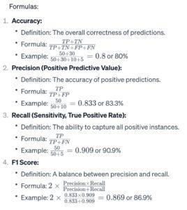
Model accuracy is a metric used to assess the performance of a class model. It measures the percentage of efficaciously predicted instances out of the overall times inside the dataset. In the context of sentiment analysis using the Naive-Bayes version, accuracy affords an average view of how properly the version is performing in classifying sentiments.
Here’s how model accuracy is calculated:
True Positives (TP): The wide variety of times where the model correctly predicts the advantageous class (e.G., effective sentiment).
True Negatives (TN): The range of instances in which the model effectively predicts the poor magnificence (e.G., negative sentiment).
False Positives (FP): The variety of instances in which the model predicts the nice magnificence, but the actual magnificence is terrible.
False Negatives (FN): The number of instances in which the version predicts the terrible magnificence, however the real magnificence is tremendous.
The accuracy is then calculated the usage of the system:
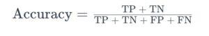
In the context of sentiment analysis, accuracy displays the overall correctness of the model in predicting whether a given textual content expresses advantageous or negative sentiment. However, it is essential to consider other metrics, inclusive of precision, do not forget, and F1 rating, specifically whilst coping with imbalanced datasets or whilst there’s a specific recognition on minimizing fake positives or fake negatives.
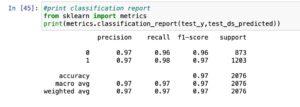
- The model is classifying with very high accuracy.
- Both average precision and recall is about 97% for identifying positive and negative sentiment document.
The high accuracy, average precision, and consider values suggest that the Naive-Bayes version is appearing nicely in classifying sentiments in the given dataset. Here’s what those metrics typically suggest:
Accuracy: The common correctness of the model in predicting sentiments. An excessive accuracy shows that a large portion of both superb and poor sentiments are efficaciously categorised.
Precision: The share of actual fine predictions amongst all instances anticipated as fine. In the context of sentiment evaluation, excessive precision means that once the model predicts an advantageous sentiment, it’s far likely to be accurate.
Recall (Sensitivity): The share of real tremendous predictions amongst all real positive instances. In the context of sentiment analysis, high remember means that the version is ideal at identifying advantageous sentiments among all the advantageous instances.
It’s vital to notice that even as accuracy is a valuable metric, precision and recollect provide extra nuanced insights while handling imbalanced datasets. For example, if the dataset has a substantially better variety of superb sentiments than bad sentiments, precision and consideration can assist in examining how well the version is performing for each sentiment elegance.
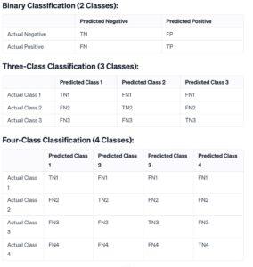
Confusion Matrix:
A confusion matrix is a desk used to assess the performance of a classification version. It summarizes the predictions made by way of a model on a dataset, evaluating them with the real effects.

Let’s delve into extra details on the inference from the confusion matrix:
Binary Classification (2 Classes):
True Negative (TN): Documents efficaciously expected as negative sentiment.
False Positive (FP): Documents incorrectly anticipated as nice sentiment (Type I error).
False Negative (FN): Documents incorrectly expected as negative sentiment (Type II mistakes).
True Positive (TP): Documents correctly expected as tremendous sentiment.
Inference:
In the binary classification case:
There are 25 instances in which high-quality sentiment documents were misclassified as negative sentiment (False Negatives).
There are 39 times where negative sentiment files were misclassified as tremendous sentiment (False Positives).
All other times are correctly categorised.
This information enables in knowledge the version’s performance, particularly in terms of errors it makes. False Positives and False Negatives are crucial metrics depending at the software and the value related to each sort of mistakes. In this example, False Negatives can be extra crucial because it way missing wonderful sentiments.
Using TF-IDF Vectorizer
Let’s complicated on using TfidfVectorizer about creating both TF (Term Frequency) vectors and TF-IDF (Term Frequency-Inverse Document Frequency) vectors:
TF Vectorizer:
When use_idf is ready to False:
TfidfVectorizer features as a TF Vectorizer.
It creates vectors primarily based on the frequency of terms (phrases) inside the document.
The vectors represent how frequently every word seems in a document.
TF-IDF Vectorizer:
When use_idf is about to True:
TfidfVectorizer functions as a TF-IDF Vectorizer.
It consists of the idea of Inverse Document Frequency (IDF).
TF-IDF considers now not simplest the frequency of a time in a report however additionally how particular or important the time is throughout all files within the corpus.
The vectors are weighted to provide better importance to phrases which can be rare across documents and lower importance to not unusual phrases.
In precis, setting use_idf to False consequences in TF vectors, whilst placing it to True outcomes in TF-IDF vectors. The choice between these depends on the specific necessities of the natural language processing mission to hand.
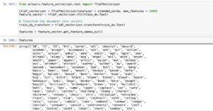
Let’s delve into the utility of Gaussian Naive Bayes for classifying files represented with the aid of TF-IDF vectors:
Gaussian Naive Bayes for TF-IDF Classification:
TF-IDF Vectors as Features:
TF-IDF vectors related to every elegance (high quality or bad sentiment) are dealt with as continuous values.
Each record’s TF-IDF vector turns into a set of capabilities for classification.
Gaussian Naive Bayes:
Gaussian Naive Bayes assumes that the functions (TF-IDF values in this example) related to every elegance are allotted according to a Gaussian (regular) distribution.
It fashions the chance of every class primarily based on the observed distribution of functions.
Gaussian Naive Bayes is suitable while dealing with non-stop-valued capabilities.
Implementation with GaussianNB:
GaussianNB from the sklearn.Naive_bayes module is used for Gaussian Naive Bayes category.
It estimates the mean and variance of every characteristic for every class based at the training records.
Classification Decision:
Given a new report’s TF-IDF vector, the version calculates the likelihood of the report belonging to each magnificence primarily based on the Gaussian distribution.
The elegance with the highest likelihood is anticipated as the very last class.
Using Gaussian Naive Bayes in this context leverages the idea that TF-IDF values follow a Gaussian distribution for powerful report classification.
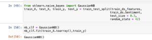
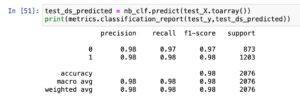
Precision, Recall, and F1-Score:
Precision:
Precision measures the accuracy of wonderful predictions made by means of the model.
In the context of sentiment analysis, a excessive precision way that after the version predicts a document as nice (1), it is correct maximum of the time.
In this case, each class (wonderful and bad sentiment) have excessive precision (0.98), indicating correct predictions.
Recall:
Recall (Sensitivity or True Positive Rate) measures the potential of the version to capture all of the superb times inside the dataset.
A excessive keep in mind indicates that the version is effective at figuring out superb instances.
In this example, each training has high don’t forget (0. Ninety seven and zero.98), displaying that the model is right at taking pictures positive sentiment instances.
F1-Score:
F1-Score is the harmonic mean of precision and recall, providing a stability between the 2 metrics.
It is especially beneficial while there’s an imbalance between the instructions.
The weighted common F1-Score is 0.98, indicating a good balance between precision and consider.
Accuracy:
Accuracy measures the overall correctness of the version predictions.
While the overall accuracy is high (0. Ninety eight), it’s critical to observe that high accuracy can be misleading, in particular in scenarios with imbalanced classes.
In real-world scenarios, wherein records may be greater various and imbalanced, excessive accuracy may not assure robust performance.
Macro and Weighted Averages:
Macro Avg:
The macro average computes metrics independently for each class and then takes the unweighted suggest.
It affords an average overall performance across instructions, treating every magnificence equally.
Weighted Avg:
The weighted average computes metrics for each magnificence and then weights them by way of the wide variety of true times for each magnificence.
It is useful whilst managing imbalanced datasets, giving more weight to the overall performance on the majority elegance.
In summary, at the same time as the presented metrics show awesome overall performance in sentiment type, it’s vital to not forget the goals and demanding situations of the real-international scenario, mainly in cases of imbalanced information.
Challenges of Text Analytics
Your factors highlight some of the demanding situations and issues in natural language processing and sentiment evaluation. Let’s elaborate on every:
Context-Specific Text:
The language used can range appreciably throughout one of a kind domain names or contexts. Movie reviews might also have exclusive sentiments expressed compared to product opinions or social media remarks.
It emphasizes the importance of area-unique schooling facts to construct a model that understands the nuances of the unique context.
Informal Language:
Informal language, consisting of slang and emoticons, poses a challenge for sentiment evaluation fashions.
Adequate schooling examples containing casual language and emoticons are critical for the model to examine and generalize successfully.
Multilingual Text:
Social media structures frequently incorporate a mix of languages, and users may additionally switch among languages inside a unmarried sentence or message.
Training facts should replicate this multilingual thing to ensure the model can handle numerous language inputs.
Sentence Structure and Sequence:
The Bag of Words (BoW) model, at the same time as powerful, disregards the sequential shape of words in a sentence.
This drawback may be addressed by thinking about n-grams, which seize sequences of n adjoining words. It facilitates maintain a few contexts information.
N-Grams:
N-grams are combinations of adjacent words in a chain (bi-grams for 2 words, trigrams for 3, etc.).
By incorporating n-grams, the version profits a better know-how of the relationships among phrases in a sentence, enhancing its capability to capture context.
In summary, constructing strong sentiment evaluation models includes addressing the specificity of the language, accommodating informality, managing multilingual text, and considering the sequential nature of language via strategies
N-Grams in Sentiment Analysis
Tokenization:
Tokenization is the procedure of breaking down a text into individual words or tokens.
Each token becomes a potential function for sentiment evaluation.
Significance of Word Sequences:
Certain expressions derive their which means from the collection of words they form.
Example: “not happy” contains a specific sentiment than studying the phrases “now not” and “satisfied” one after the other.
Introduction to N-Grams:
N-grams are contiguous sequences of n words. They seize the relationships and context between phrases.
Bigrams: Pairs of consecutive phrases (e.G., “no longer happy”).
Trigrams: Sequences of 3 consecutive words.
Enhancing Context Understanding:
By treating consecutive phrases as single functions, the version gains a better knowledge of the context in which sure words or sentiments seem.
It allows address the dilemma of the Bag of Words version, which would not keep in mind phrase order.
Example:
Consider the sentence “This movie is not desirable at all.”
Unigrams (individual phrases): [‘This’, ‘movie’, ‘is’, ‘not’, ‘good’, ‘at’, ‘all’]
Bigrams (consecutive pairs): [(‘This’, ‘movie’), (‘movie’, ‘is’), (‘is’, ‘not’), (‘not’, ‘good’), (‘good’, ‘at’), (‘at’, ‘all’)]
Trigrams (consecutive triples): [(‘This’, ‘movie’, ‘is’), (‘movie’, ‘is’, ‘not’), (‘is’, ‘not’, ‘good’), (‘not’, ‘good’, ‘at’), (‘good’, ‘at’, ‘all’)]
Implementation:
While growing features for sentiment analysis, incorporating n-grams permits the model to don’t forget the contextual that means conveyed by way of phrase sequences.
Incorporating n-grams presents a more nuanced expertise of language shape and improves the version’s ability to seize sentiment in context.
- Write a new custom analyzer *get_stemmed_tokens()* , which splits the sentences and stems the phrases from them before creating *n-grams*.
- This code block eliminates non-aphabetic characters and then applies stemming.
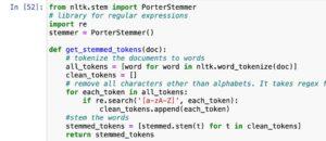
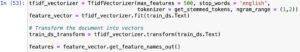
In this case, the get_stemmed_tokens custom tokenizer is used with TfidfVectorizer, and the ngram_range is ready to (1, 2) to create each unigram (unmarried phrases) and bigrams (consecutive pairs of words) as features. The ensuing TF-IDF matrix considers the context of words in the sentences with the aid of incorporating n-grams.
Build the model using n-grams
- Split dataset to 70:30 ratio for creating training and test datasets and then apply *BernoulliNB* for classification.
- Models predict the test set and classification report.
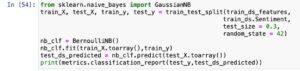
The recall for identifying documents (with label 1) have increased to almost 1.0.
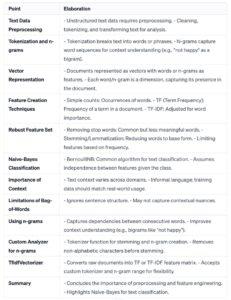
- Text data is unstructured data and needs extensive pre-processing before applying models.
- Documents or sentences can be tokenized into unigrams or n-grams for building features.
- The documents can be represented as vectors with words or n-grams as features.
- The vectors can be creating using simple counts, TF (Term Frequency) or TF-IDF values.
- A robust set of features can be created by removing stop words and applying stemming or lemmatization.
- Number of features can also be limited by selecting only features with higher frequencies.
- Naive-Bayes classification models (BernoulliNB) are the most widely used algorithm for classifying texts.
Conclusion
NLP case studies combine computational linguistics—rule-based modeling of human language—with statistical, machine learning, and deep learning models. With the help of these technologies, computers can now process human language in the form of text or voice data and fully “understand” what is being said or written, including the speaker’s or writer’s intentions and sentiments. Homonyms, homophones, sarcasm, idioms, metaphors, exceptions to the rules of grammar and usage and changes in sentence structure are just a few examples of the irregularities in human language that take humans years to learn but that programmers must teach natural language-driven applications to recognize and understand accurately from the beginning if those applications are to be helpful.

The details being provided about Natural Language Processing (NLP) and its functioning detailing every view and aspect of its working is something very informative and helpful. Along with these details information regarding the use of NLP in daily life makes it very insightful taking you to the pulse of the matter. The blog contains almost every point that one should know about the topic, besides that under every subtopic its description will leave no doubts on your mind to be unsolved.
The blog provides wide and wholesome data on the NLP on such a short note and in brief words that it will eventually become helpful in every parameter of judgment and will turn out to be the most useful blog for this topic.
The details provided about Natural Language Processing (NLP) and how it works, detailing each view and aspect of their work, is very informative and helpful. Along with this detailed information on how to use NLP in daily life, it is very enlightening in bringing you to the heart of the matter. The blog contains almost every point that one should know about the topic, moreover its description on each sub-topic will leave no doubt in words that eventually it will be helpful in every parameter of judgment and will turn out to be the most useful blog on this topic .
It is very enlightening and beneficial to read the information provided about Natural Language Processing (NLP) and how it operates in detail. Along with these specifics, the information about how NLP is used in everyday life makes it very illuminating and gets right to the heart of the matter. The blog essentially covers every aspect of the subject that one should be aware of, and each subtopic’s description will clear up any confusion you might have.
The blog offers comprehensive and well-rounded information on NLP in such a condensed space and with such clear language that it will eventually prove to be beneficial in all areas of judgment and will emerge as the most helpful blog on the subject.
The information being provided about Natural Language Processing (NLP) and how it functions, describing every aspect and viewpoint of its operation, is unquestionably instructive and beneficial. With these specifics and information about how NLP is used during the day, it becomes incredibly perceptive, bringing you right up to the heart of the matter. In addition to covering practically all relevant information, the blog’s descriptions of each subtopic will leave no questions in your mind unanswered.
The site offers comprehensive and well-rounded information about NLP in such a concise manner and with such simple language that it will prove to be the most beneficial blog for this material in the long run.