SQL Basic to Advance
History of SQL:
SQL, short for Structured Query Language, has a history rooted in the 1970s when IBM developed the System R project. It aimed to create a database management system that could handle and manipulate structured data efficiently. As part of System R, IBM introduced a language called Structured English Query Language (SEQUEL), which later evolved into SQL The name “SEQUEL” was already taken by another company. The creators of the language didn’t want to get sued, so they changed the name to ‘SQL’. SQL is a backronym for “Structured Query Language.” The language was influenced by Edgar F. Codd’s relational model, which introduced the concept of organizing data into tables with relationships. Over time, SQL became the standard language for interacting with relational databases and was standardized by ANSI and ISO. Today, SQL is widely adopted and utilized in various database systems, enabling organizations to manage and analyze structured data effectively.
Let’s first understand the Data modeling and database:
What is Data Modeling?
Data Modeling is a critical step in defining data structure, creating data models to describe associations and constraints for reuse. Data Modeling is the conceptual design or plan for organizing data. It visually represents data with diagrams, symbols, or text to visualize relationships.
Enhancing data analytics, data modeling assures uniformity in nomenclature, rules, semantics, and security. Regardless of the application, the emphasis is on the arrangement and accessibility of the data.
What are the Advantages of Data Modelling
The following are the essential advantages of Data Modelling:
- The data modeling helps us choose the right data sources to populate the model.
- The Data Model improves communication throughout the company.
- The data model aids in the ETL process’s documentation of the data mapping.
- We can use data modeling to query the database’s data and generate various reports based on the data. Data modeling supports data analysis through reports.
Data Modeling Terminology:
- Entity: Entities are the objects or items in the business environment for which we need to store data. Defines what the table is about. For example, in an e-commerce system, entities can be Customers, Orders, or Products.
- Attributes: Attributes provide a way to structure and organize the data within an entity. They represent the specific characteristics or properties of an entity. For instance, attributes of a customer entity can include Name, Address, and Email.
- Relationship: Relationships define how entities are connected or associated with each other. They explain the interactions and dependencies between entities. For example, the relationship between Customers and Orders represents that a customer can place multiple orders.
- Reference Table: A reference table is used to resolve many-to-many relationships between entities. It transforms the relationship into one-to-many or many-to-one relationships. For instance, in a system with Customers and Products, a reference table called OrderDetails can be used to link customers with the products they have ordered.
- Database Logical Design: It refers to designing the database within a specific data model of a database management system. It involves creating the structure, relationships, and rules of the database at a conceptual level.
- Logical Design: Logical design involves the creation of keys, tables, rules, and constraints within the database. It focuses on the logical structure and organization of data without considering specific implementation details.
- Database Physical Design: It encompasses the decisions related to file organization, storage design, and indexing techniques for efficient data storage and retrieval within the database.
- Physical Model: The physical model is a representation of the database that considers implementation-specific details such as file formats, storage mechanisms, and index structures. It translates the logical design into an actual database implementation.
- Schema: A schema refers to the complete description or blueprint of the database. It defines the structure, relationships, constraints, and permissions associated with the database objects.
- Logical Schema: A logical schema represents the theoretical design of a database. It is typically created during the initial stages of database design, similar to drawing a structural diagram of a house. It helps visualize the relationships and organization of
The database entities and attributes.
Levels of Data Abstraction:
Data modeling typically involves several levels of abstraction, including:
Conceptual level: This is the highest level of data abstraction. It’s about what data you need to store, and how it relates to each other. You can use diagrams or other visual representations to show this.
Example: You might decide that you need to store data about customers, products, and orders. You might also decide that there is a relationship between customers and orders, and between products and orders.
Logical level: This is the middle level of abstraction. It’s about how the data will be stored and organized. You can use data modeling languages like SQL or ER diagrams to show this.
Example: You might decide to store the data in a relational database. You might create tables for customers, products, and orders, and define relationships between the tables.
Physical level: The physical level is the most basic or lowest data abstraction. It concerns the particulars of how the data will be kept on disc. Data types, indexes, and other technical information fall under this category.
Example: You might decide to store the data in a specific database server, and use a specific data type for each column. You might also decide to create indexes to improve the performance of queries.
What are the perspective of data modeling?
-
Network Model:
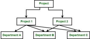
- The Network Model represents data as interconnected records with predefined relationships. It allows for many-to-many relationships and uses a graph-like structure. For example, in a company’s database, employees can work on multiple projects, and each project can have multiple employees assigned to it. The Network Model connects employee records to project records through relationship pointers, enabling flexible relationships.
Check the below image:
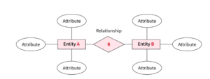
2. Entity-Relationship (ER) Model:
- The ER Model represents data using entities, attributes, and relationships. Entities are real-world objects, attributes describe their properties, and relationships depict connections between entities. For instance, in a university database, entities could be Students and Courses, with attributes like student ID and course name. Relationships, such as “Student enrolls in Course,” illustrate the associations between entities.
Check the below Image:
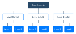
3. Hierarchical Model:
- Data is arranged in a tree-like structure with parent-child relationships using the hierarchical model. There is one parent and several children per record. Consider the organizational hierarchy, where the CEO is at the top and is followed by the managers, employees, and department heads. These hierarchical links are graphically represented by the hierarchical model, allowing top-to-bottom or bottom-to-top navigation.
Check the below image:
4. Relational Model:
- The Relational Model organizes data into tables consisting of rows and columns. It creates relationships between tables using primary and foreign keys. For example, in a customer and orders scenario, customer information is stored in one table, while order details are stored in another. The Relational Model connects the tables using a shared key, like a customer ID, to link relevant records.
Check the below image.
| OrderID | CustomerID | OrderDate |
TotalAmount |
|
|
1001 |
1 | → | 2023-07-01 |
250.00 |
|
1002 |
2 | → | 2023-07-02 |
150.00 |
|
1003 |
1 | → | 2023-07-03 |
300.00 |
|
1004 |
4 | → | 2023-07-04 |
200.00 |
What is Database?
A database is like a digital warehouse where data is stored, organized, and managed efficiently. Database is a physical or digital storage system that implements a specific data model. Database is the actual implementation of that design, where the data is stored and managed. It acts as a central hub for information, making it easier to access and analyze data.
What are the Components of DBMS (Database Management System)
- Data: Data is the raw information stored in a database, such as customer details, product information, or financial records. It can be in different formats like text, numbers, dates, or images.
- Tables: Tables are like virtual spreadsheets within a database. They have rows and columns, where each row represents a specific record or instance, and each column represents a particular piece of data. For example, a table for customers may have columns like ID, Name, Address, and Contact.
- Relationships: Relationships define how tables are connected within a database. They establish associations based on shared data elements. For instance, a customer’s ID in one table can be linked to their orders in another table. This helps maintain data consistency and enables efficient data retrieval.
- Queries: Queries are like search commands that allow users to extract specific data from the database. Users can search, filter, and sort data based on the criteria they specify. For example, a query can be used to find all customers who made a purchase in the last month.
A Quick Overview of Different Types of Databases
- Relational Databases (RDBMS): Relational databases separate data into rows and columns and tables, and they build associations between tables using keys. They are frequently used in business applications that manipulate data using Structured Query Language (SQL). Oracle, MySQL, and Microsoft SQL Server are a few examples.
- NoSQL Databases: NoSQL databases are Non-relational databases that offer flexible data models without using a fixed schema. They can manage enormous amounts of semi- or unstructured data. MongoDB, Cassandra, and Couchbase are a few examples.
- Object-Oriented Databases: Similar to object-oriented programming, OODBs store data as objects. They are helpful for programs that deal with intricate interactions and data structures. Examples are ObjectDB and db4o.
- Hierarchical Databases: Hierarchical databases organize data in a tree-like structure, where each record has a parent-child relationship. They are suitable for representing hierarchical relationships, such as organization structures. IMS (Information Management System) is an example of a hierarchical database.
- Network Databases: Network databases are similar to hierarchical databases but allow for more complex relationships. They use a network model where records can have multiple parent and child records. CODASYL DBMS (Conference on Data Systems Languages) is an example of a network database.
- Graph Databases: Graph databases store data in a graph structure with nodes and edges. They are designed to represent and process relationships between data points efficiently. They are commonly used for social networks, recommendation engines, and network analysis. Examples include Neo4j and Amazon Neptune.
- In-Memory Databases: In-memory databases store data primarily in memory, resulting in faster data access and processing compared to disk-based databases. They are suitable for applications that require high-speed data operations. Examples include Redis and Apache Ignite.
- Time-Series Databases: Time-series databases are optimized for storing and retrieving time-stamped data, such as sensor data, financial data, or log files. They provide efficient storage and retrieval of time-series data for analysis. Examples include InfluxDB and Prometheus.
RDBMS vs DBMS: Everything You Need to Know
Although they are both software system used to manage databases, DBMS (Database Management System) and RDBMS (Relational Database Management System) have different qualities.
Why required DBMS?
A Database Management Systems is required to efficiently manage the flow of data within an organization. It handles tasks such as inserting data into the database and retrieving data from it.
The Database Management Systems ensures the consistency and integrity of the data, as well as the speed at which data can be accessed.
Why required RDMS?
Similarly, a Relational Database Management System (RDBMS) is required when we want to manage data in a relational manner, using tables and relationships. It helps in reducing data duplication and maintaining the integrity of the database. Relational Database Management System ensures that data is stored in a structured manner, allowing for efficient querying and retrieval.
Difference Between DBMS and RDBMS – Detailed Comparisons:
|
DBMS |
RDBMS |
| Applications using DBMS save data in files. | RDBMS applications store data in a tabular form. |
| No relationship between data. |
Related data stored in the form of table. |
| Normalization is not present. | Normalization is present. |
| Distributed databases are not supported by DBMS. | RDBMS supports distributed database. |
| It works with small quantity of data. | It works with large amount of data. |
| Security is less | More security measures provided. |
| Low software and hardware necessities | Higher software and hardware necessities. |
| Examples: XML Window Registry, Forxpro, dbaseIIIplus etc. | Examples: PostgreSQL, MySQL, Oracle, Microsoft Access, SQL Server etc. |
What is Normalization in SQL?
The process of normalization data in a database ensures data integrity by removing duplication. A database must be split up into various tables, and linkages must be established between them. Different levels of normalization exist, such as 1NF (First Normal Form), 2NF (Second Normal Form), 3NF (Third Normal Form), and BCNF (Boyce-Codd Normal Form)
1NF (First Normal Form):
In 1NF, each column in a table contains only atomic values, meaning it cannot be further divided. There should be no repeating groups or arrays of values within a single column. Each row in the table should be uniquely identifiable. Here’s an example:
Original Table:
| CustomerID | Name | Phone no. |
|
1 |
Jia ria |
8978847383 |
|
2 |
John Doe |
7899748899, 8899278299 |
|
3 |
Smith tie |
9877382892 |
1NF Table:
| CustomerID | Name | Phone no. |
|
1 |
Jia ria | 8978847383 |
|
2 |
John Doe |
7899748899 |
|
3 |
Smith tie |
9877382892 |
|
4 |
John Doe |
8899278299 |
2NF (Second Normal Form):
In 2NF, the table is already in 1NF, and each non-key column is dependent on the entire primary key. If there are partial dependencies, those columns should be moved to a separate table. Here’s an example:
Original Table:
| OrderID | ProductID | ProductName | Category | Price |
|
1 |
1 | Laptop | Electronics |
1000 |
|
2 |
2 | Smartphone | Electronics |
800 |
|
3 |
3 | Laptop | Electronics |
900 |
2NF Tables:
Table 1: Products
| ProductID | ProductName | Category |
|
1 |
Laptop |
Electronics |
|
2 |
Smartphone |
Electronics |
Table 2: Orders
| OrderID | ProductID | Price |
|
1 |
1 |
1000 |
|
2 |
2 |
800 |
|
3 |
1 |
900 |
3NF (Third Normal Form):
In 3NF, the table is already in 2NF, and there are no transitive dependencies. Non-key columns should not depend on other non-key columns. If there are such dependencies, those columns should be moved to a separate table. Here’s an example:
Original Table:
| CustomerID | OrderID | ProductID | Price | CustomerName | CustomerEmail |
|
1 |
1 | 1 | 1000 | John Doe | |
|
2 |
2 | 2 | 800 | Jane Smith | |
|
3 |
3 | 1 | 900 | John Doe |
3NF Tables:
Table 1: Customers
| CustomerID | CustomerName | CustomerEmail |
|
1 |
John Doe | |
|
2 |
Jane Smith | |
|
3 |
John Doe |
Table 2: Products
| ProductID | ProductName |
|
1 |
Laptop |
|
2 |
Smartphone |
Table 3: Orders
| OrderID | CustomerID | ProductID | Price |
|
1 |
1 | 1 |
1000 |
|
2 |
2 | 2 |
800 |
|
3 |
3 | 1 |
900 |
BCNF (Boyce-Codd Normal Form):
BCNF is an advanced form of normalization that addresses certain anomalies that can occur in 3NF. It ensures that there are no non-trivial functional dependencies of non-key attributes on a candidate key. Achieving BCNF involves decomposing tables further if necessary.
Binary Relationships:
A binary relationship exists when two different relationships are involved. Accordingly, every entity in the connection has a unique association with one entity in the other entity. For instance, a passport can only be issued to one individual, and a person is only allowed to have one passport at a time. An illustration of a one-to-one relationship might be this.
Cardinality:
Cardinality refers to the number of instances of an entity that can be associated with an instance of another entity. There are four types of cardinalities:
One-to-One
Each instance of one entity can only be linked to one instance of the other, and vice versa, in a one-to-one relationship. It is commonly used to represent one-to-one things in the actual world, such a person and their passport, and is the strictest kind of relationship.
Example: A person can have only one passport, and a passport can be issued to only one person.
One-to-Many
A one-to-many relationship means that each instance of one entity can be associated with multiple instances of the other entity, but each instance of the other entity can only be associated with one instance of the first entity. This is a common type of relationship, and it is often used to represent hierarchical relationships in the real world, such as a parent and their children.
Example: A customer can place multiple orders, but each order can only be placed by one customer.
Many-to-One
An entity in A is associated to no more than one entity in B in this particular cardinality mapping. Or, we may say that any number (zero or more) of entities or things in A can be connected to a unit or thing in B.
Example: A single surgeon performs many operations in a specific institution. A many-to-one relationship is one of these relationships.
Many-to-Many
A many-to-many relationship means that each instance of one entity can be associated with multiple instances of the other entity, and each instance of the other entity can also be associated with multiple instances of the first entity. This is the most common type of relationship, and it is often used to represent relationships where the order of the entities does matter, such as a student and their courses.
Example: A student can take multiple courses, and each course can be taken by multiple students.
Introduction to SQL (Structured Query Language):
The computer programming language SQL (Structured Query Language) was developed especially for managing and changing relational databases. It provides commands and statements to connect to databases, retrieve and modify data, construct database structures, and perform numerous data tasks. More details are provided below:
What Is SQL, and How Is It Used?
According to its definition and intended application, SQL is a declarative language utilized for relational database management. By constructing queries, it enables users to interact with databases to access, alter, and manage structured data. No matter what database management system is used underneath, SQL provides a standardized and efficient method for working with databases.
What is SQL For Data Science? Database Definition for Beginners?
Due to its adaptability and efficiency in maintaining relational databases, SQL is frequently used in data science and analytics. The main justifications for SQL’s high value are as follows:
- The core activities of inserting, updating, and deleting data in relational databases are made available to data professionals via SQ. It gives a simple and effective method for changing data.
- SQL gives customers the ability to get particular data from relational database management systems. Users can provide criteria and conditions to retrieve the desired information by creating SQL queries.
- SQL is useful for expressing the structure of stored data. Users can define the structure, data types, and relationships of database tables as well as add, change, and delete them.
- SQL gives users the ability to handle databases and their tables efficiently. In order to increase the functionality and automation of database operations, it facilitates the construction of views, stored procedures, and functions.
- SQL gives users the ability to define and edit data that is kept in a relational database. Data constraints can be specified by users, preserving the integrity and consistency of the data.
- Data Security and Permissions: SQL has tools for granting access to and imposing restrictions on table fields, views, and stored procedures. Giving users the proper access rights promotes data security.
SQL Constraints
- Specific Rules for the data in a table can be defined using constraints in SQL.
- The data that can be entered into a table is restricted by SQL constraints. It assures the reliability and accuracy of the data inserted in the table. The action is stopped if there is a violation/breach between the constraint and the data action.
- Column-level or table-level SQL constraints are both possible. Table-level restrictions apply to the entire table, while column-level constraints just affect the specified column.
Restrictions on SQL functions are frequently applied:
- NOT NULL: A column cannot have a NULL value by using the NOT NULL flag.
- UNIQUE: A unique value makes sure that each value in a column is distinct.
- PRIMARY KEY: A NOT NULL and UNIQUE combination. Identifies each table row in a unique way.
- FOREIGN KEY: Prevent acts that would break linkages between tables.
- CHECK – Verifies if the values in a column meet a certain requirement.
- DEFAULT: If no value is specified, DEFAULT sets a default value for the column.
- CREATE INDEX – Used to easily create and access data from the database.
NOT NULL constraint
- A column may by default contain NULL values.
- A column must not accept NULL values according to the NOT NULL constraint.
- This forces a field to always have a value, thus you cannot add a value to this field while adding a new record or updating an existing record.
- Syntax:
CREATE TABLE Persons (
ID int NOT NULL,
LastName varchar(255) NOT NULL,
FirstName varchar(255) NOT NULL,
price int);
Check Constraint:
- The value range that can be entered into a column is restricted by the CHECK constraint.
- Only specific values will be permitted for a column if you define a CHECK constraint on it.
- A table’s CHECK constraint can be used to restrict the values in specific columns based on the values of other columns in the same row.
Example: Create check constraint:
CREATE TABLE employee (
ID int NOT NULL,
LastName varchar(255) NOT NULL,
FirstName varchar(255),
Age int,
CHECK (Age>=18));
Working with DEFAULT Constraints in SQL:
- A column’s default value is set using the DEFAULT constraint.
- If no alternative value is supplied, the default value will be appended to all new records.
- Example: Create Default.
CREATE TABLE EMPLOYEE (
ID int NOT NULL,
LastName varchar(255) NOT NULL,
FirstName varchar(255),
Age int,
City varchar(255) DEFAULT ‘LONDON’);
- By utilizing operations like GETDATE, the DEFAULT constraint can also be utilized to insert system data ()
The Most Popular Types of Keys in SQL
We’ll talk about keys and the many types that exist in SQL Server. Let’s define keys to get this topic started.
Types of keys – SQL Release?
In RDBMS systems, keys are fields that take part in the following operations on tables:
- To establish connections between two tables.
- To keep a table’s individuality.
- To maintain accurate and consistent data in the database.
- Possibly speed up data retrieval by enabling indexes on column (s).
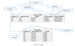
What are the Different Types of SQL Keys: Example and Uses That SQL Server supports:
- Candidate Key
- Primary Key
- Unique Key
- Alternate Key
- Composite Key
- Super Key
- Foreign Key
- Candidate Key:
- A candidate key is a table’s primary key that has the potential to be chosen. There may be several candidate keys in a table, but only one can be chosen to serve as the main key.
Example: The candidate keys are License Number, Employee Id, , and Passport Number.
- Primary Key
- The table’s primary key was chosen as a candidate key to uniquely identify each record. Primary keys maintain unique values throughout the column and do not permit null values. Employee Id is the primary key of the Employee table in the example above. In SQL Server, a heap table’s main key automatically builds a clustered index (a table which does not have a clustered index is known as a heap table). A table’s nonclustered primary key can also be defined by explicitly specifying the kind of index.
- A table can have only one primary key, in SQL Server, the primary key can be defined using SQL commands below:
- CRETE TABLE statement (at the time of table creation) – In this case, system defines the name of primary key
- ALTER TABLE statement (using a primary key constraint) – User defines the name of the primary key
Example: Employee_Id is a primary key of Employee table.
- Unique Key
- Similar to a primary key, a unique key prevents duplicate data from being stored in a column. In comparison to the primary key, it differs in the following ways:
- One null value may be present in the column.
- On heap tables, it by default creates a nonclustered index.
- Alternate Key
- The alternate key is a potential primary key for the table that has not yet been chosen.
- For instance, other keys include License Number and Passport Number.
- Composite Key
- Each row in a table is uniquely identified by a composite key, sometimes referred to as a compound key or concatenated key. A composite key’s individual columns might not be able to identify a record in a certain way. It may be a candidate key or a primary key.
- Example: To uniquely identify each row in the salary database, Employee Id and Salary Month Year are merged. Each entry cannot be individually identified by the Employee Id or Salary Month Year columns alone. The Employee Id and Salary Month Year columns in the Salary database can be used to build a composite primary key.
- Super Key
- A super key is a group of columns from which the table’s other columns derive their functional dependence. Each row in a table is given a unique identification by a collection of columns. Additional columns that are not strictly necessary to identify each row uniquely may be included in the super key. The minimal super keys, or subset of super keys, are the primary key and candidate keys.
- In the previous example, the Employee table’s Employee Id column served as a super key for the Employee Table because it was sufficient to uniquely identify each row of the table.
- As an illustration, consider the following: “Employee Id,” “Employee Id, Employee Name,” “Employee Id, Employee Name, Address,” etc.
An Introductory SQL Syntax: A Tutorial How to Write SQL Queries:
SQL syntax is the set of rules that govern how SQL statements are written. It is a language that is used to interact with relational databases. SQL statements can be used to create, read, update, and delete data in a database.
The basic syntax of a SQL statement is:
- Keyword [parameter_1, parameter_2, …]
The keyword is the name of the SQL statement. The parameters are the values that are passed to the statement.
For example, the following is a SELECT statement that selects the Name and Department ID columns from the Students table:
SELECT Name, Department ID
FROM Students;
The keyword is SELECT, and the parameters are Name and Department ID.
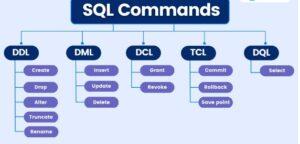
An Introduction to SQL Commands
- The set of guidelines governing the writing of SQL statements is known as SQL syntax. The SQL commands CREATE, DROP, INSERT, and others are employed in the SQL language to do the necessary activities.
- A table receives instructions from SQL commands. It is used to perform some Tasks on the database. Additionally, it is utilized to carry out particular duties, functions, and data inquiries. Table creation, data addition, table deletion, table modification, and user permission setting are just a few of the activities that SQL is capable of.
The five main categories into which these SQL commands fall are as follows:
- Data Definition Language (DDL)
- Data Query Language (DQL)
- Data Manipulation Language (DML)
- Data Control Language (DCL)
- Transaction Control Language (TCL)
What is Data Definition Language (DDL)?
- The SQL statements that can be used to specify the database schema make up DDL, or Data Definition Language. It is used to create and modify the structure of database objects in the database and only works with descriptions of the database schema. Although data cannot be created, modified, or deleted with DDL, database structures can. In most cases, a typical user shouldn’t use these commands; instead, they should use an application to access the database.
DDL Commands & Syntax List:
CREATE: Create the database or its objects using the CREATE (like database, table, index, function, views, store procedure, and triggers).
SYNTAX:
CREATE DATABASE database_name
CREATE TABLE table_name (
column1 datatype,…);
DROP: Use the DROP command to remove objects from the database.
SYNTAX:
— For database
DROP DATABASE database_name;
— For table
DROP TABLE table_name;
ALTER: This is used to change the database’s structure.
SYNTAX
ALTER TABLE table_name
ADD column_name datatype;
ALTER TABLE table_name
DROP COLUMN column_name;
ALTER TABLE table_name
MODIFY column_name datatype;
TRUNCATE: This function is used to eliminate every record from a table, along with any spaces set aside for the records.
SYNTAX:
TRUNCATE TABLE table_name;
RENAME: This command is used to rename an existing database object.
SYNTAX
–– rename table
RENAME table_name TO new_table_name;
— renaming a column
ALTER TABLE table_name
RENAME COLUMN column_name TO new_column_name;
DQL (Data Query Language)
- DQL is a sublanguage of SQL that is used to query data from a database.
- It is a declarative language, which means that you tell the database what you want, not how to get it.
- DQL statements are made up of keywords, operators, and values.
- Some common DQL keywords include SELECT, FROM, WHERE, and ORDER BY.
- SYNTAX
- select *
- from customer_orders
- where customer_id = 100;
DML (Data Manipulation Language)
The majority of SQL statements are part of the DML which is used to manipulate data that is present in databases. It is part of the SQL statement in charge of managing database and data access. Essentially, DML statements and DCL statements belong together.
DML commands list:
- INSERT: Data is inserted into a table using the INSERT command.
SYNTAX
INSERT INTO table_name (column1, column2,..)
VALUES (value1, value2,..);
- UPDATE: A table’s existing data is updated using UPDATE.
SYNTAX:
UPDATE table_name
SET column1 = new_value1, …
WHERE condition;
- DELETE: Delete records from a database table using the DELETE command.
SYNTAX:
DELETE FROM table_name
WHERE condition;
- LOCK: Concurrency under table management.
SYNTAX:
LOCK TABLE table_name IN lock_mode;
- CALL: Call a Java or PL/SQL subprogram.
- SYNTAX:
CALL subprogram_name
- EXPLAIN PLAN: It outlines the data access route.
DCL (Data Control Language)
DCL comprises commands such as GRANT and REVOKE which largely deal with the rights, permissions, and other controls of the database system.
List of DCL commands:
GRANT: This command gives users access privileges to the database.
Syntax:
GRANT SELECT, UPDATE ON MY TABLE TO SOME USER, ANOTHER USER;
REVOKE: This command withdraws the user’s access privileges supplied by using the GRANT command.
Syntax:
REVOKE SELECT, UPDATE ON MY TABLE FROM USER1, USER2;
TCL (Transaction Control Language)
A group of tasks are combined into a single execution unit using transactions. Each transaction starts with a particular defined task and is completed once every activity in the group has been properly executed. The transaction fails if any of the task is unsuccessful. Therefore, a transaction has only two outcomes: success or failure. Here, you may learn more about transactions. As a result, the following TCL commands are used to manage how a transaction is carried out:
TCL commands list:
- BEGIN: Opens a transaction with BEGIN
- Syntax:
- COMMIT: Completes a Transaction.
- Syntax:
- COMMIT;
- Rollback: When an error occurs, a transaction is rolled back.
- Syntax:
- ROLLBACK;
- SAVEPOINT: Creates a transactional save point.
- Syntax:
- The SAVEPOINT NAME;
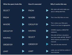
SQL query Execution Order
SQL Statements: The Complete List With Examples:
The specific queries or operations entered into the database using the SQL language are known as SQL statements. They are employed to access, modify, or administer data stored in database tables. Keywords, expressions, clauses, and operators make up SQL statements.
SELECT STATEMENT: MySQL
- To get data from the database, use the SELECT statement.
- The information received is kept in a result table known as the result-set.
For example, in the code below, we’re choosing a row from a table called employees for a field called name.
INPUT:
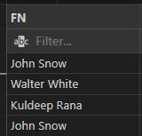
SELECT FullName
FROM employees;
OUTPUT:

SELECT *
All of the columns in the table we are searching will be returned when SELECT is used with an asterisk (*).
INPUT:
SELECT *
FROM employees;
OUTPUT:

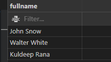
SELECT DISTINCT
- If there are duplicate records, SELECT DISTINCT will only return one of each; otherwise, it will provide data that is distinct.
- The code below would only retrieve rows from the Employees table that had unique names.
INPUT:
SELECT DISTINCT(fullname)
FROM employees;
OUTPUT:
SELECT INTO
The data supplied by SELECT INTO is copy from one table to another.
SELECT * INTO customer_orders
FROM employees;
Aliases (AS):
- Aliases are frequently used to improve the readability of column names.
- An alias only exists while that query is running.
- By using the AS keyword, an alias is produced.
- For instance, we’re renaming the name column in the code below to fullname: AS renames a column or table with an alias that we can choose.
INPUT:
SELECT FullName as FN
FROM employees;
OUTPUT:
Alias for Tables
SELECT o.OrderID, o.OrderDate, c.CustomerName
FROM Customers AS c, Orders AS o
WHERE c.CustomerName=’Around the Horn’ AND c.CustomerID=o.CustomerID;
From
FROM identifies the table from which we are obtaining our data.
SELECT *
FROM EMPLOYEES
SQL WHERE Clause
- Records can be filtered using the WHERE clause.
- It is used to exclusively extract records that meet a certain requirement.
- The WHERE clause is a part of an SQL SELECT statement that tells the database which rows to return. It uses a variety of operators to compare values in the database to values that you specify.
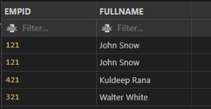
INPUT:
SELECT *
FROM EMPLOYEES
WHERE EMPID=321
OUTPUT:

NOTE: Single quotes must be used around text values in SQL. However, quotations should not be used around numeric fields:
SQL Operators: Types, Syntax and Examples in the WHERE Clause:
|
Operator |
Description |
|
= |
Equal |
|
> |
Greater than |
|
< |
Less than |
|
>= |
Greater than or equal to |
|
<= |
less than or equal to |
| <>, != |
Not equivalent. Note: This operator may be written as ! In some SQL versions. |
|
between |
Within a specific range |
|
like |
Look for patterns |
|
in |
to designate a column’s potential values in numerous ways |
Tricky SQL Interview Questions For Where Claus:
- Can you use aggregate functions in the WHERE clause?
No, you cannot use aggregate functions directly in the WHERE clause. Instead, you typically use them in the HAVING clause to filter the results of aggregate queries.
- What is the difference between WHERE and HAVING clauses?
The WHERE clause is used to filter rows before they are grouped or aggregated, while the HAVING clause is used to filter grouped or aggregated results. The HAVING clause can use aggregate functions, unlike the WHERE clause.
- Can you use multiple conditions in the WHERE clause?
Yes, you can combine multiple conditions using logical operators such as AND and OR. For example:
WHERE condition1 AND condition2
WHERE condition1 OR condition2
- What happens if you use a column alias in the WHERE clause?
The WHERE clause is evaluated before the SELECT clause, so you cannot use column aliases defined in the SELECT clause directly in the WHERE clause. However, you can use the original column name or wrap the query in a subquery.
- Remember, the WHERE clause is a powerful tool for filtering and retrieving specific data from a table based on conditions. It allows you to narrow down the result set and perform complex queries to meet your specific requirements.
And, or, and not operators in SQL:
- Operators like AND, OR, and NOT can be used with the WHERE clause.
- To filter records based on multiple criteria, use the AND , OR operators:
- If every condition that is divided by AND is TRUE, the AND operator displays a record.
- If any of the terms divided by OR is TRUE, the OR operator outputs a record.
- If the condition(s) is/are NOT TRUE, the NOT operator displays a record.
AND – INPUT:
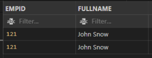
SELECT EMPID, FULLNAME
FROM EMPLOYEES
WHERE EMPID=121 AND FULLNAME=”John Snow”:
Output:
OR – OPERATOR
INPUT:
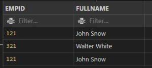
SELECT EMPID,
FULLNAME
FROM EMPLOYEES
WHERE EMPID = 121
OR FullName = “Walter White”;
OUTPUT:
NOT OPERATOR
INPUT:
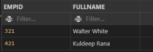
SELECT EMPID, FULLNAME
FROM employees
WHERE NOT EMPID=121
OUTPUT:
SQL ORDER BY Keyword
- The result set can be sorted in either ascending or descending order using the ORDER BY keyword.
- Records are typically sorted using the ORDER BY keyword in ascending order. Use the DESC keyword to sort the records in descending order.
Example: Ascending Order by
Input:
SELECT EMPID, FULLNAME
FROM employees
ORDER BY FullName
Output:
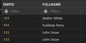
Example: Descending Order by
Input:
SELECT EMPID, FULLNAME
FROM employees
ORDER BY FullName DESC
Output:
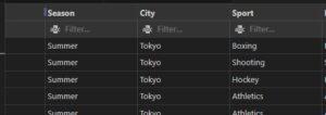
Example of ORDER BY Several Columns
In this example as you can see SQL Statement selected all column from athlete_event3 table and order by with multiple column.
Input:
SELECT *
FROM athlete_events3
ORDER BY Season, City DESC
Output:
INSERT INTO STATEMENT
To add new records to a table, use the INSERT INTO statement.
INSERT INTO Syntax
There are two methods to format the INSERT INTO statement:
- Specify the values to be inserted together with the column names.
- You do not need to provide the column names in the SQL query if you are adding values to every column of the table. However, make sure the values are arranged in the same order as the table’s column headings. In this case, the syntax for INSERT INTO would be as follows:
INPUT:
INSERT INTO EMPLOYEES(EMPID, FULLNAME, MANAGERID, DATEOFJOINING, CITY)
VALUES(333,”JAY RAO”,999,2019-03-20,”LONDON”)
OUTPUT:

Additionally, you can insert data entry to certain columns.
IS NULL OPERATOR
Testing for empty values is done with the IS NULL operator (NULL values).
To check for non-empty values, use the IS NOT NULL operator (NOT NULL values).
- Example: The SQL statement below lists every employee whose “city” field has a NULL value:
SELECT FullName, EmpId, city
FROM EMPLOYEES
where city is null;
SQL DELETE Statement
Existing records in a table can be deleted using the DELETE statement.
- Reminder: Take care while eliminating records from a table! In the DELETE statement, pay attention to the WHERE clause. Which record(s) should be removed is specified by the WHERE clause. All records in the table will be erased if the WHERE clause is left off.
Example: Check below , delete statement deleteing city toronto from employees table.
DELETE
FROM EMPLOYEES
where city =’Toronto’;
Output: Toronto city deleted.

What is SQL LIMIT Clause & Where you should use?
The number of rows to return is specified using the LIMIT clause.
On huge tables with tens of thousands of records, the LIMIT clause is helpful. Performance may be affected if many records are returned.
- The SELECT TOP clause is not supported by all database management systems. In contrast to Oracle, which employs FETCH FIRST n ROWS ONLY and ROWNUM, MySQL supports the LIMIT clause to restrict the number of records that are selected.
- EXAMPLE: from employees table only 2 records display
INPUT:
SELECT *
FROM EMPLOYEES
LIMIT 2;
OUTPUT:

SQL UPDATE Statement
The existing records in a table can be changed using the UPDATE command.
- When updating records in a table, take caution! In the UPDATE statement, pay attention to the WHERE clause. The record(s) to be modified are specified by the WHERE clause. The table’s records will all be updated if the WHERE clause is left off!
UPDATE A multiple Of Records
How many records are updated is determined by the WHERE clause.
Note: When updating records, exercise caution. ALL records will be updated if the WHERE clause is not included!
Example: Update records fullname rana where city is London
UPDATE employees
SET FULLNAME=’RANA’
WHERE CITY=’London’;
Output:

What is Aggregate function in SQL with example:
A number of aggregation functions exist in SQL that can be used to conduct calculations on a collection of rows and return a single value. Here are a few aggregation functions that are frequently used:
SUM()= Determines the total of a column or expression using SUM().
for instance:
SELECT SUM(ORDER_AMOUNT)
FROM CUSTOMER_ORDERS;
Output:

AVG()= Determines the average of a column or phrase using AVG().
for instance:
SELECT AVG(ORDER_AMOUNT)
FROM CUSTOMER_ORDERS;
Output:

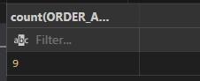
COUNT() = Returns the number of rows in a table or the number of rows that meet a condition using the COUNT() function.
Example:
SELECT COUNT(ORDER_AMOUNT)
FROM CUSTOMER_ORDERS;
Output:
MAX()= The MAX() function displays the highest value in a column or expression.
Example:
SELECT MAX(ORDER_AMOUNT)
FROM CUSTOMER_ORDERS;
Output:

MIN()= Function display the lowest value in the column.
SELECT MIN(ORDER_AMOUNT)
FROM CUSTOMER_ORDERS;
Output:

Types Of Operators in SQL with Example:
Like Operator in SQL:
To look for a specific pattern in a column, use the LIKE operator in a WHERE clause.
Two wild cards are frequently combined with the LIKE operator:
The percent sign (%) denotes a character or many characters.
The underscore character (_) stands for a single character.
- Please take note that MS Access substitutes an asterisk (*) for the percent sign (%) and a question mark (?) for the underscore ( ).
- Additionally, you can combine the underscore and the % sign!
|
Operator |
Description |
|
WHERE FULLNAME LIKE ‘a%’ |
Searches for any values beginning with “a,” |
|
WHERE FULLNAME LIKE ‘%a’ |
Searches for values ending in “a.” |
|
WHERE FULLNAME LIKE ‘%or%’ |
identifies any values that contain the word “or” anywhere. |
|
WHERE FULLNAME LIKE ‘_r%’ |
in the second position is done by using the WHERE |
|
WHERE FULLNAME LIKE ‘a_%’ |
Finds any values that begin with “a” and have at least two characters in length using the WHERE |
|
WHERE FULLNAME LIKE ‘a__%’ |
Search any values that start with “a” and are at least 3 characters in length. |
|
WHERE FULLNAME LIKE ‘a%o’ |
Search any values that start with “a” and ends with “o”. |
Example: Find fullname starts with w from employees table
SELECT *
FROM EMPLOYEES
WHERE FULLNAME LIKE ‘W%’;
Output:

IN SQL Operator
You can define several values in a WHERE clause by using the IN operator.
The numerous OR conditions are abbreviated as the IN operator.
Syntax:
SELECT column_name(s)
FROM table_name
WHERE column_name IN (value1, value2, …);
OR
SELECT column_name(s)
FROM table_name
WHERE column_name IN (SELECT STATEMENT);
Example: Select all records where city in california and new delhi.
SELECT *
FROM employees
WHERE CITY IN (‘CALIFORNIA’,’NEW DELHI’)
Output:

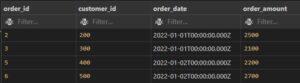
BETWEEN OPERATOR in SQL:
- The BETWEEN operator chooses values from a predetermined range. The values could be text, integers, or dates.
- The BETWEEN operator includes both the begin and finish variables.
BETWEEN EXAMPLE: select order amount between 2100 to 2900 from customer orders
SELECT *
FROM customer_orders
WHERE ORDER_AMOUNT BETWEEN 2100 AND 2900;
Output:
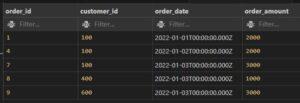
Not between Operator In SQL:
Example: select order amount which not in range 2100 to 2900 from customer orders table.
SELECT *
FROM customer_orders
WHERE ORDER_AMOUNT NOT BETWEEN 2100 AND 2900
Output:
BETWEEN with IN Operator In SQL:
Example: select all records where order amount range between 2100 and 2900 and also order id 1,4,8
SELECT *
FROM customer_orders
WHERE ORDER_AMOUNT NOT BETWEEN 2100 AND 2900
AND ORDER_ID IN(1,4,8)
Output:

SQL Between- Tricky SQL interview Questions and Answers:
- Does the BETWEEN operator include the boundary values?
Yes, the BETWEEN operator includes the boundary values. It is an inclusive range operator, so values equal to value1 or value2 will be included in the result.
- Can the BETWEEN operator be used with non-numeric data types?
Yes, the BETWEEN operator can be used with non-numeric data types such as dates, strings, or timestamps. It compares the values based on their inherent order or alphabetic sequence.
- What happens if value1 is greater than value2 in the BETWEEN operator?
The BETWEEN operator still functions correctly even if value1 is greater than value2. It will return rows where the column value falls within the specified range, regardless of the order of value1 and value2.
- Can you use the NOT operator with the BETWEEN operator?
Yes, you can use the NOT operator to negate the result of the BETWEEN operator. For example:
WHERE column_name NOT BETWEEN value1 AND value2
- Can you use the BETWEEN operator with NULL values?
No, the BETWEEN operator cannot be used with NULL values because NULL represents an unknown value. Instead, you can use the IS NULL or IS NOT NULL operators to check for NULL values.
- Can you use the BETWEEN operator with datetime values and timestamps?
Yes, the BETWEEN operator can be used with datetime values and timestamps to filter rows within a specific date or time range.
Remember, the BETWEEN operator provides a convenient way to filter rows based on a range of values. It is widely used for various data types and allows for inclusive range comparisons. Understanding its behavior and nuances will help you accurately retrieve the desired data from your database.
What are joins and types of joins in SQL with examples
Data is kept in several tables that are connected to one another in relational databases like SQL Server, Oracle, MySQL, and others via a common key value. As a result, it is frequently necessary to combine data from two or more tables into one results table. The SQL JOIN clause in SQL Server makes this simple to do. A JOIN clause is used to combine rows from those tables based on a shared column between two or more of the tables. They allow you to retrieve data from multiple tables in a single query, based on common data points. Here’s a detailed explanation of SQL joins:
joins and types of SQL joins with examples:
- Inner join/ Equijoin
- Left join
- Right join
- Full outer join
- Cross join/ Cartesian Join
- Self join
- Natural join
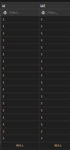
- Inner join/ Equijoin:
If the criteria is met, the INNER JOIN keyword selects all rows from both tables. By merging all rows from both tables that meet the requirement—that is, have the same value for the shared field—this keyword will provide a result set. Inner joins are a useful way to combine data from two tables where there is a relationship between the two tables.
Here are some of the benefits of using inner joins:
- They can be used to get a more complete picture of a set of data.
- They can be used to identify customers who have placed an order.
- They can be used to join tables that have different schemas.
Here are some of the limitations of using inner joins:
- They can return less data than other types of joins.
- They can be inefficient if there are a lot of rows in the two tables that do not have matching values.
- The join condition is typically an equality comparison between the related columns in the two tables.
- You can use table aliases to simplify the syntax and improve readability.
- You can join more than two tables by extending the join operation using additional INNER JOIN clauses.
- Check the below image.
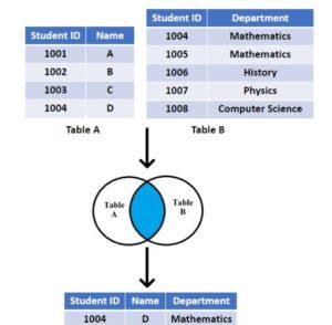
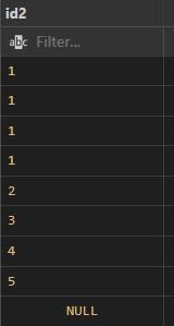
Example: First create table T1, and T2.
CREATE TABLE t1 (id INT);
CREATE TABLE t2 (id2 INT);
Insert values:
INSERT INTO t1 (id) VALUES (1), (1), (1), (1), (2), (3), (NULL);
INSERT INTO t2 (id2) VALUES (1), (1), (1), (1), (2), (3), (4), (5), (NULL);
Table- T1 Table – T2
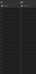
Input:
SELECT * FROM t1
INNER JOIN t2 ON t1.id = t2.id2;
Output:
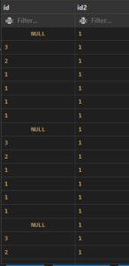
2. Right join:
This join gives back all the rows from the table on the right side of the join as well as any matching rows from the table on the left. The result-set will include null for any rows for which there is no matching row on the left. RIGHT OUTER JOIN is another name for RIGHT JOIN. Similar to LEFT JOIN is RIGHT JOIN.
In simple language,
- All rows from the right table are returned by the right join.
- The result will exclude any rows that are present in the left table but not the right table.
- Limitations: Complex queries: When using RIGHT JOINs in complex queries involving multiple tables, it can be challenging to maintain clarity and understand the relationship between tables. Careful consideration of table order and join conditions is necessary to produce accurate results.
- Code readability: RIGHT JOINs, especially in more complex queries, can make the SQL code less readable and harder to interpret.
Check the below image.
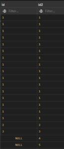
Example:
SELECT * FROM t1
RIGHT JOIN t2 ON t1.id = t2.id2;
Output:
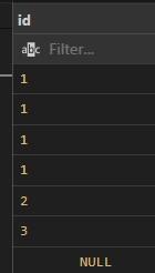
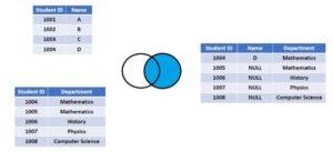
3. Left join:
The rows that match for the table on the right side of the join are returned along with all of the rows from the table on the left side of the join. The result-set will include null for all rows for which there is no matching row on the right side. LEFT OUTER JOIN is another name for LEFT JOIN. Left joins are a useful way to get all the data from one table, even if there is no matching data in another table.
Here are some of the benefits of using left joins:
- They can be used to get a complete overview of a set of data.
- They can be used to identify customers who have not yet placed an order.
- They can be used to join tables that have different schemas.
Here are some of the limitations of using left joins:
- They can return a lot of data, which can make it difficult to analyze.
- They can be inefficient if there are a lot of rows in the right table that do not have a matching row in the left table.
Check the below image.
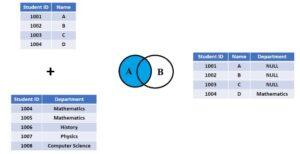
Example: Left join
SELECT * FROM t1
LEFT JOIN t2 ON t1.id = t2.id2;
Output:
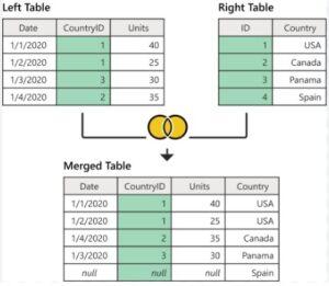
4. Full Outer Join in SQL:
By combining the results of both LEFT JOIN and RIGHT JOIN, FULL JOIN produces the result-set. The rows from both tables are all included in the result-set. The result-set will contain NULL values for the rows where there was no match. Full outer joins are a useful way to get all the data from two tables,his can be helpful for getting a complete overview of a set of data.
Here are some of the benefits of using full outer joins:
- They can be used to get a complete overview of a set of data.
- They can be used to identify customers who have not yet placed an order.
- They can be used to identify orders that have not yet been assigned to a customer.
Here are some of the limitations of using full outer joins:
- They can return a lot of data, which can make it difficult to analyze.
- They can be inefficient if there are a lot of rows in the two tables that do not have matching values.
what are benefits of cross join in sql:
Cartesian product: A CROSS JOIN generates a Cartesian product of the two tables involved, combining every row from the first table with every row from the second table. This can be useful in scenarios where you need to explore all possible combinations between two sets of data.
Data expansion: CROSS JOIN can be used to create additional rows, especially when working with dimension tables or reference tables that have a small number of rows. This expansion can be beneficial for creating test data or generating comprehensive reports.
Limitations of CROSS JOIN:
- Result set size: The result set of a CROSS JOIN can grow rapidly, especially when joining large tables or multiple tables. The Cartesian product generates a number of rows equal to the product of the number of rows in the joined tables, which can lead to a significant increase in the dataset’s size.
- Performance impact: Due to the potential for a large result set, a CROSS JOIN operation can have a performance impact on the database. It can consume significant resources and take longer to execute compared to other types of joins.
Check the below image:
Example:
SELECT * FROM t1
Cross JOIN t2;
Output:
5. Natural Join in SQL:
The NATURAL JOIN is a type of join operation in SQL that combines tables based on columns with the same name and data type. It automatically matches columns between tables and returns only the matching rows. Here’s a detailed explanation of the NATURAL JOIN, and the difference between NATURAL JOIN and CROSS JOIN:
Synatx:
SELECT * FROM t1
NATURAL JOIN t2;
Benefits of NATURAL JOIN:
- Simplicity: NATURAL JOIN simplifies the join operation by automatically matching columns with the same name and data type between the joined tables. It eliminates the need to explicitly specify the join conditions, reducing the complexity and potential for errors in the query.
- Readability: NATURAL JOIN can enhance code readability as it reflects the inherent relationship between tables based on column names. It improves query comprehension and makes the code more intuitive and self-explanatory.
Limitations of NATURAL JOIN:
- Ambiguous column names: If the joined tables contain columns with the same name but different meanings, using NATURAL JOIN can lead to confusion or produce incorrect results. It relies solely on column names and data types, disregarding any semantic differences.
- Lack of flexibility: NATURAL JOIN provides limited control over the join conditions. It may not suit complex scenarios where more specific or custom join conditions are required.
- Performance implications: NATURAL JOIN might impact performance, especially when joining large tables or in cases where indexing is not optimized for the matching columns.
What is the difference between cross join and natural join:
- CROSS JOIN: A CROSS JOIN, or Cartesian join, combines every row from the first table with every row from the second table, resulting in a Cartesian product. It does not consider any column matching or relationships between tables. It generates a large result set that includes all possible combinations between the joined tables.
- NATURAL JOIN: A NATURAL JOIN combines tables based on columns with the same name and data type. It automatically matches the columns between tables and returns only the matching rows. It considers the column names as the join condition, without explicitly specifying it.
6. Self Join in SQL:
A self join is a type of join operation in SQL that allows you to join a table with itself. It is useful when you want to compare rows within the same table or establish relationships between different rows in the table.
Syntax:
SELECT columns
FROM table1 AS t1
JOIN table1 AS t2 ON t1.column = t2.column;
Benefits of Self Joins:
- Comparing related data: Self joins allow you to compare and analyze related data within the same table. For example, you can compare sales data for different time periods or evaluate hierarchical relationships within organizational data.
- Establishing relationships: Self joins enable you to establish relationships between rows within a table. This is common in scenarios where data has a hierarchical structure, such as an employee table with a self-referencing manager column.
- Simplifying complex queries: Self joins simplify complex queries by enabling you to consolidate related information in a single result set. This can help in performing calculations, aggregations, or generating reports based on self-related data.
Limitations of Self Joins:
- Performance impact: Self joins can have a performance impact, especially on large tables or when the join condition is not optimized. It is important to ensure proper indexing on the relevant columns for improved performance.
- Code complexity: Self joins can make the SQL code more complex and potentially harder to read and understand. It is crucial to provide clear aliases and document the purpose and logic of the self join for easier comprehension and maintenance.
Tricky questions on joins in SQL server:
What is a self join, and when would you use it?
A self join is a join operation where a table is joined with itself. It is useful when you want to compare rows within the same table or establish relationships between different rows in the table, such as hierarchical data or comparing related records.
Can you perform a JOIN operation without specifying the JOIN condition?
No, specifying the join condition is essential for performing a join operation in SQL. It defines the relationship between the tables being joined and determines how the rows are matched.
How does a LEFT JOIN differ from a RIGHT JOIN?
A LEFT JOIN returns all rows from the table on the left and the matching rows from the table on the right. On the other hand, RIGHT JOIN returns all rows from the table on the right and the matching rows from the table on the left.
What is the result of joining a table with itself using a CROSS JOIN?
Joining a table with itself using a CROSS JOIN, also known as a Cartesian join, results in the Cartesian product of the table. It combines every row from the table with every other row, resulting in a potentially large result set.
Can you JOIN more than two tables in a single SQL query?
Yes, it is possible to join more than two tables in a single SQL query. This is often required when you need to combine data from multiple tables to retrieve the desired information.
How can you simulate a FULL OUTER JOIN in a database that does not support it?
In databases that do not support a FULL OUTER JOIN, a FULL OUTER JOIN can be simulated by combining a LEFT JOIN and a RIGHT JOIN using the UNION operator.
What is the difference between a natural join and an equijoin?
A natural join is a join operation that automatically matches columns with the same name and data type between the joined tables. An equijoin, on the other hand, is a join operation that explicitly specifies the equality condition between columns in the joined tables.
Can you use the WHERE clause to perform a JOIN operation?
While it is possible to use the WHERE clause to filter rows in a join operation, it is generally recommended to use the JOIN condition in the ON clause for specifying the relationship between the tables being joined.
How can you exclude rows that match in a JOIN operation?
To exclude rows that match in a JOIN operation, you can use an OUTER JOIN (LEFT JOIN or RIGHT JOIN) and check for NULL values in the columns of the non-matching table. Rows with NULL values indicate that they exist in one table but not in the other.
Can you join tables with different data types in SQL?
Yes, it is possible to join tables with different data types in SQL as long as the join condition is based on compatible data types. SQL will automatically perform necessary data type conversions if possible.
How can you optimize the performance of a JOIN operation?
To optimize the performance of a JOIN operation, you can ensure that the join columns are properly indexed, use appropriate join types (e.g., INNER JOIN instead of CROSS JOIN), and apply relevant filtering conditions to reduce the result set size.
Is it possible to JOIN tables based on non-matching columns?
Yes, it is possible to join tables based on non-matching columns by using conditions other than equality in the JOIN clause, such as using greater than or less than operators.
What are the implications of using a Cartesian product (CROSS JOIN)?
The Cartesian product can result in a large result set, especially if the joined tables have many rows. It can consume significant resources, impact query performance, and lead to unintended data duplication if not used carefully.
Can you JOIN tables that have different column names?
Yes, it is possible to join tables that have different column names. In such cases, you can specify the column names explicitly in the join condition using aliases or by using the ON clause to specify the relationship between the columns with different names.
What is GROUP BY Statement in SQL:
In database management systems like SQL, the group by clause is a strong tool for categorizing rows of data based on one or more columns. It enables data aggregation and summarization, delivering insightful data and facilitating effective analysis. The COUNT(), MAX(), MIN(), SUM(), and AVG() aggregate functions are frequently used with the GROUP BY statement to group the result set by one or more columns. Although this feature has many advantages, it also has some drawbacks and particular applications.
Benefits of Group By Statement in SQL:
- Data Summarization: Grouping enormous datasets according to specified criteria enables us to summarize them. It makes it possible to compute several summary statistics for each group, including counts, averages, sums, minimums, maximums, and more. Understanding the broad traits and patterns in the data is made easier by this summary.
- Simplified Data Analysis: Group by streamlines the analysis process by combining relevant data. It aids in the discovery of patterns, trends, and connections in the data. A clearer image is created by grouping data according to pertinent criteria, which also facilitates efficient decision-making.
Restrictions for Group By Statement in SQL:
- Data Loss: Only aggregated results are shown when using the Group by clause; the original detailed information is lost. This could be a drawback if specific data points or individual records must be scrutinized for more in-depth research. In some circumstances, complex computations or unique aggregations might be necessary, which the Group by clause might not directly handle.
- Syntax:
SELECT column_name(s)
FROM table_name
WHERE condition
GROUP BY column_name(s)
ORDER BY column_name(s);
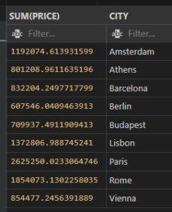
- Example: sum up price for each city wise from aemf2 table.
SELECT SUM(PRICE), CITY
FROM aemf2
GROUP BY CITY;
Output:
What is HAVING Clause in SQL With Example:
Since the WHERE keyword cannot be used with aggregate functions, the HAVING clause was added to SQL
Utilizing aggregate function-based conditions, the HAVING clause in SQL is used to restrict the results of a query. To filter grouped data, it is frequently combined with the GROUP BY clause. After grouping and aggregation, the HAVING clause enables you to apply criteria to the grouped data. In most cases, the HAVING clause is used in conjunction with the GROUP BY clause.
The advantages of HAVING Clause in SQL include:
- Grouped Data Filtering: The HAVING clause’s capacity to filter grouped data depending on conditions is its main advantage. You can use it to specify complicated conditions that incorporate aggregate functions and column values to limit the result set to only the groups that match particular requirements.
- Flexible Aggregate Filtering: The HAVING clause allows for flexible aggregate filtering of data. It enables you to specify constraints on an aggregate function’s output.
The having clause in SQL has some restrictions.
- Order of Evaluation: The GROUP BY and aggregate procedures are assessed before the HAVING clause. Because they are not yet available during the evaluation of the HAVING condition, column aliases and aggregate functions established in the SELECT clause cannot be used in the HAVING clause.
- Performance Impact: When working with huge datasets, the HAVING clause may have an effect on performance.
Syntax:
SELECT column1, column2,…
FROM table
GROUP BY column1, column2,…
HAVING condition;
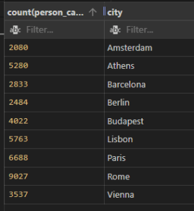
Example: count the person capacity who have grater then 2 with each city from aemf2 table.
SELECT count(person_capacity),city
FROM aemf2
group by City
having count(person_capacity)>2;
Output:
Difference Between Group by and Having clause in SQL:
Purpose:
GROUP BY: The GROUP BY clause is used to group rows together based on one or more columns. It creates distinct groups of data based on the specified columns.
HAVING: The HAVING clause is used to filter the grouped data after the grouping and aggregation have taken place. It applies conditions to the result of aggregate functions.
Usage:
GROUP BY: The GROUP BY clause is used in conjunction with aggregate functions to perform calculations and summarizations on the grouped data.
HAVING: The HAVING clause is used to filter the grouped data based on conditions involving aggregate functions. It narrows down the result set to only those groups that satisfy the specified conditions.
Placement:
GROUP BY: The GROUP BY clause is placed after the FROM and WHERE clauses but before the ORDER BY clause (if used) in a SQL query.
HAVING: The HAVING clause is placed after the GROUP BY clause in a SQL query. It follows the GROUP BY clause and precedes the ORDER BY clause (if used).
Evaluation:
GROUP BY: The GROUP BY clause operates on the original rows of data and creates groups based on the specified columns. It does not filter or remove any rows from the original dataset.
HAVING: The HAVING clause operates on the grouped data after the GROUP BY and aggregation steps. It applies conditions to the aggregated results and filters out groups that do not satisfy the specified conditions.
Tricky SQL Having Clause Interview Questions with Answers
Q: What is the difference between the WHERE clause and the HAVING clause?
A: The WHERE clause is used to filter rows before grouping and aggregation, while the HAVING clause is used to filter the grouped data after grouping and aggregation.
Q: Can you use the HAVING clause without the GROUP BY clause?
A: No, the HAVING clause is always used in conjunction with the GROUP BY clause. It operates on the grouped data resulting from the GROUP BY clause.
Q: What happens if you include a column in the SELECT statement that is not in the GROUP BY clause?
A: In most SQL implementations, including a column in the SELECT statement that is not in the GROUP BY clause will result in an error. However, some databases allow it with specific configuration settings.
Q: Can you have multiple HAVING clauses in a single SQL query?
A: No, a SQL query can have only one HAVING clause. However, you can use multiple conditions within the HAVING clause using logical operators such as AND and OR.
Q: How is the ORDER BY clause different from the HAVING clause?
A: The ORDER BY clause is used to sort the final result set based on specified columns, while the HAVING clause is used to filter the grouped data based on conditions involving aggregate functions.
Q: Is it possible to use aggregate functions in the HAVING clause?
A: Yes, the HAVING clause is specifically designed to work with aggregate functions. It allows you to apply conditions to the results of aggregate functions.
Q: Can you use the GROUP BY clause without the HAVING clause?
A: Yes, the GROUP BY clause can be used independently to group rows of data without applying any conditions or filters.
Q: What is the order of execution for the GROUP BY and HAVING clauses in a SQL query?
A: The GROUP BY clause is executed first to create the groups, followed by the HAVING clause, which filters the groups based on the specified conditions.
Q: What happens if you interchange the positions of the GROUP BY and HAVING clauses in a SQL query?
A: Swapping the positions of the GROUP BY and HAVING clauses will result in a syntax error. The GROUP BY clause should always precede the HAVING clause.
Q: Can you use non-aggregated columns in the HAVING clause?
A: No, non-aggregated columns should be used in the GROUP BY clause. The HAVING clause operates on aggregated results and conditions should involve aggregate functions.
Union and Union all in SQL:
To concatenate the result-set of two or more SELECT statements, use the UNION operator.
- Within UNION, all SELECT statements must have an identical number of columns.
- Similar data types must also be present in the columns.
- Every SELECT statement’s columns must be in the same order.
- Syntax:
- SELECT column_name FROM table1
- UNION
- SELECT column_name FROM table2;
UNION ALL Syntax
- By default, the UNION operator only chooses distinct values. To allow duplicate values, use UNION ALL:
- SELECT column_name FROM table1
- UNION ALL
- SELECT column_name FROM table2;
Difference Between Union and Union all in SQL:
Duplicate Rows:
UNION: The UNION operator removes duplicate rows from the final result set. It compares all columns in the result sets and eliminates duplicates.
UNION ALL: The UNION ALL operator does not remove duplicate rows. It includes all rows from each SELECT statement, even if there are duplicates.
Performance:
UNION: The UNION operator implicitly performs a sort operation to remove duplicates. This additional sorting process can impact performance, especially when dealing with large result sets.
UNION ALL: The UNION ALL operator does not perform any sorting or elimination of duplicates, making it generally faster than UNION.
Result Set Size:
UNION: The size of the result set produced by the UNION operator may be smaller than the sum of the individual result sets due to the removal of duplicate rows.
UNION ALL: The size of the result set produced by the UNION ALL operator is equal to the sum of the individual result sets, including duplicate rows.
How to Use ANY and ALL Operators in SQL:
You can compare a single column value to a variety of other values using the ANY and ALL operators.
The ANY Operator in SQL
Using the ANY operator provides a Boolean value in the form of TRUE if ANY of the values returned by the subquery satisfy the condition ANY denotes that the condition will hold true if the operation holds for ANY of the values in the range. It can be used with comparison operators such as =, >, <, >=, <=, <> (not equal).
Syntax:
SELECT column_name
FROM table_name
WHERE column_name operator ANY
(SELECT column_name
FROM table_name
WHERE condition);
Operator ALL:
provides a boolean value that, when combined with SELECT, WHERE, and HAVING statements, returns TRUE if ALL of the subquery values satisfy the criteria.
ALL denotes that the operation must be true for each and every value in the range for the condition to be true.
Syntax:
SELECT ALL column_name
FROM table_name
WHERE condition;
What Are The Differences between SQL ANY and ALL Operators:
Comparison Logic:
ANY: The ANY operator returns true if the comparison is true for at least one value in the set.
ALL: The ALL operator returns true if the comparison is true for all values in the set.
Usage in Subqueries:
ANY: The ANY operator compares the single value with each value in the set individually.
ALL: The ALL operator compares the single value with all values in the set collectively
What Are MySQL Functions with Examples:
There are several built-in functions in MySQL.
This reference includes sophisticated MySQL functions as well as string, numeric, date, and other data types.
String Functions:
String data types can be manipulated and operated on using string functions in SQL. They offer a range of options for extracting, changing, and editing string values. Here is a thorough description of several typical SQL string functions:
- CONCAT(str1, str2, …):
- combines one or more strings into one.
Example:
SELECT CONCAT(‘Hello’, ‘ ‘, ‘World’)
Output: Returns ‘Hello World’.
- LENGTH(str):
- returns the length of a string, or the number of characters.
Example:
SELECT LENGTH(‘Hello’)
Output: 5 is returned by
- UPPER(str):
- a string is changed to uppercase.
Example:
SELECT UPPER(“hello”)
Output: “HELLO”
- LOWER(str):
- lowercases a string of characters.
Example: The result of SELECT LOWER(‘WORLD’)
SELECT LOWER(‘WORLD’)
Output: is “world”.
- SUBSTRING(str, start, length):
- extracts a substring with a specified length and beginning at a particular location from a string.
Example:
SELECT SUBSTRING(‘Hello World’, 7, 5)
Output: returns ‘World’.
- STRAIGHT(str, length):
- gets a certain amount of characters from a string’s left side.
Example:
SELECT LEFT(‘Database’, 4)
Output: ‘Data’.
- Wrong(str, length):
- a string’s right side is emptied of a certain amount of characters.
For instance,
SELECT RIGHT(“Table,” “3”)
Output: gives “ble.”
- TRIM([characters FROM] str]):
- Removes certain characters or leading and trailing spaces from a string.
Example:
SELECT TRIM(‘Hello ‘)
Output: is “Hello”.
- REPLACE(str, replacement value, search value):
- replaces a substring with a new substring wherever it appears in the string.
Example:
SELECT REPLACE(‘Hello, World!’, ‘World’, ‘SQL’)
Output: Hello, SQL!
- STRING(str, search str):
- returns the location of a substring’s first occurrence within a string.
Example:
SELECT INSTR(‘Hello World’, ‘World’)
Output: There are 7 results from the query.
- REVERSE(str):
- Reverses the order of characters in a string.
- LEFT():
- Returns sub string from the left of given size or characters.
Example:
SELECT LEFT(‘MYSQL IS’, 5);
Output: MYSQL
- RIGHT():
- Returns a sub string from the right end of the given size.
Example:
SELECT RIGHT(‘MYSQL.COM’, 4)
Output: .com
Date Functions:
In SQL, date functions are used to perform various operations on date and time data types. They provide capabilities for manipulating, extracting, and formatting date and time values.
- CURRENT_DATE():
- Returns the current date.
Example:
SELECT CURRENT_DATE()
Output: gives the current date.
- CURRENT_TIME():
- Gives the current time.
Example:
SELECT CURRENT_TIME()
Output: the current time.
- CURRENT_TIMESTAMP():
- Gives both the current date and time.
Example:
SELECT CURRENT_TIMESTAMP()
Output: current date and time.
- EXTRACT(part FROM date):
- Extracts a part of (year, month, day, hour, minute, second, etc.) from a date.
Example:
SELECT EXTRACT(YEAR FROM ‘2023-07-14’)
Output: returns 2023.
- DATEADD(datepart, interval, date):
- Adds a specific interval of time to a date.
Example:
SELECT DATEADD(MONTH, 3, ‘2022-01-01’)
Output: returns ‘2022-04-01’.
- DATEDIFF(datepart, start_date, end_date):
- Calculates the difference between two dates as per mentioned date part (year, month, day, etc.).
Example:
SELECT DATEDIFF(DAY, ‘2022-01-01’, ‘2022-01-31’)
Output: returns 30.
- DATEPART(datepart, date):
- Gives the mentioned part (year, month, day, hour, minute, second, etc.) of a date.
Example:
SELECT DATEPART(HOUR, ‘2022-01-01 09:30:45’)
Output: returns 9.
- DATE_FORMAT(date, format):
- Change a date according to the specified format.
Example:
SELECT DATE_FORMAT(‘2022-01-01’, ‘%Y-%m-%d’)
Output: returns ‘2022-01-01’.
- TO_CHAR(date, format):
- Converts a date to a string using the specified format.
Example:
SELECT TO_CHAR(‘2022-01-01’, ‘YYYY-MM-DD’)
Output: returns ‘2022-01-01’.
- DATE_TRUNC(part, date):
- Truncates a date to the specified part (year, month, day, hour, minute, second, etc.).
Example:
SELECT DATE_TRUNC(‘MONTH’, ‘2022-01-15’)
Output: returns ‘2022-01-01’.
- ADD_MONTHS(date, months):
- Adds the specified number of months to a date.
Example:
SELECT ADD_MONTHS(‘2022-01-01’, 3)
Output: Returns ‘2022-04-01’.
- LAST_DAY(date):
- Gives the last day of the month for a given date.
Example:
SELECT LAST_DAY(‘2022-02-15’)
Output: returns ‘2022-02-28’.
- DAYNAME(date):
- Gives the name of the day for a given date.
Example:
SELECT DAYNAME(‘2022-01-01’)
Output: returns ‘Saturday’.
- MONTHNAME(date):
- Gives the name of the month for a given date.
Example:
SELECT MONTHNAME(‘2022-01-01’)
Output: Returns ‘January’.
- NOW():
- Gives the current date and time.
Example: SELECT NOW() Gives the current date and time.
When to Use Advance Window Function in SQL:
Advance SQL window functions are analytical operations on a group of rows known as a “window” or “frame” within the result set. They enable the execution of calculations and aggregations on a per-row basis while taking the window’s context into account. A thorough explanation of numerous SQL window functions is provided below, along with a sample code: but let’s first understand what is difference between aggregation function and window function.
In SQL, sets of rows in a table can be calculated using both aggregate functions and window functions. The methods they use to organise and interpret the data vary, though.
Aggregate functions:
- Calculation scope: Aggregate functions operate on a set of rows and return a single value for the entire set.
- Grouping: They are typically used with the GROUP BY clause to partition the data into groups and calculate a result for each group.
- Result granularity: Aggregate functions collapse multiple rows into a single result. For example, SUM, AVG, COUNT, MAX, and MIN are aggregate functions.
- Usage: They are used to obtain summary statistics or perform calculations such as calculating the total sales per category, average salary per department, or counting the number of orders per customer.
Syntax:
SELECT department, AVG(salary) AS average_salary
FROM employees
GROUP BY department;
Window functions:
- Calculation scope: Window functions perform calculations on a “window” or a subset of rows within a result set.
- Ordering: They are typically used with the ORDER BY clause to define the window’s ordering within the result set.
- Result granularity: Window functions retain the individual rows in the result set but can calculate values based on the window’s defined scope.
- Usage: They are used to compute values that are related to the current row but involve other rows in the result set. Examples of window functions include RANK, ROW_NUMBER, LAG, LEAD, and SUM with the OVER clause.
HOW to Use Window function in SQL With Example:
The OVER clause, which specifies the window’s borders and ordering, is frequently combined with window functions in SQL programming.
SYNTAX:
function_name([arguments]) OVER (
[PARTITION BY partition_expression]
[ORDER BY order_expression [ASC|DESC]]
[ROWS/RANGE frame_clause]
)
- function_name: Window function name you can use, such as ROW_NUMBER, SUM, AVG, etc.
- arguments: Its optional arguments that the window function For example, SUM(column_name) would calculate the sum of the specified column.
- PARTITION BY: Optional clause that divides the rows into partitions or groups based on one or more expressions. The window function is applied separately to each partition.
- ORDER BY: Optional clause that specifies the order in which the rows within each partition should be processed by the window function. It can use one or more columns and can be sorted in ascending (ASC) or descending (DESC) order.
- ROWS/RANGE frame_clause: Optional clause that defines the window frame or the subset of rows within each partition over which the window function operates.
- ROW_NUMBER(): Each row in a window is given a distinct sequential number using the ROW NUMBER() function.
Example:
SELECT ROW_NUMBER()OVER(ORDER BY PRICE DESC) as row_no, Price
FROM aemf2
Output:
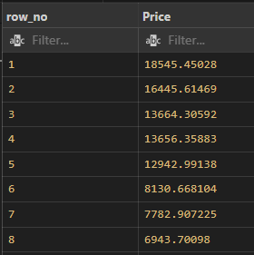
2. RANK():
- Gives each row in a window a rank, leaving gaps for tied values.
Example:
SELECT RANK()OVER(ORDER BY PRICE DESC) as row_no, Price
FROM aemf2;
3. DENSE_RANK():
- Gives each row in a window a rank, leaving no gaps for tied values.
Example:
SELECT DENSE_RANK()OVER(ORDER BY PRICE DESC) as row_no, Price
FROM ;
4. NTILE():
- Divides a window’s rows into a predetermined number of groups or “tiles.”
Example:
SELECT NTILE()OVER(ORDER BY PRICE DESC) as row_no, Price
FROM ;
5. LAG():
- Accesses a previous row’s value within a window.
Example:
SELECT PRICE,LAG(PRICE)OVER(ORDER BY DAY DESC) as row_no, Price
FROM aemf2 ;
Output:
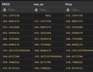
6. LEAD():
- Accesses the value of a subsequent row within a window.
Example:
SELECT PRICE,LEAD(PRICE)OVER(ORDER BY DAY DESC) as row_no, Price
FROM aemf2 ;
Output:
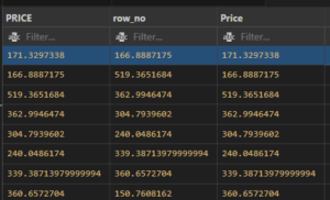
7. FIRST_VALUE():
- Accesses a previous row’s value within a window.
Example:
SELECT FIRST_VALUE(PRICE)OVER(ORDER BY DAY DESC) as FIRST_V, Price
FROM aemf2 ;
Output:
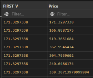
8. PERCENT_RANK():
- Accesses a previous row’s value within a window.
Example:
SELECT Sales, PERCENT_RANK() OVER (ORDER BY Sales) AS PercentileRank
FROM SalesData;
What is Common Table Expression (CTE) IN SQL With Example
Known as a Common Table Expression (CTE) in SQL, a temporary named result set may be referred to within a query. Having the ability to build a subquery and utilize it more than once within a single query might help make complex queries easier to comprehend and maintain. A detailed explanation of CTE is provided below, along with an example:
A CTE’s two constituent parts, the anchor member and the recursive member, are defined by the WITH clause (optional for recursive queries). The anchor member of the CTE serves as its foundation, while the recursive member builds upon it through iterative processing.
Benefits of using CTE in SQL:
- Improved Readability: CTEs make complex queries easier to understand by breaking them into logical sections. This improves code readability and maintainability.
- Code Reusability: CTEs can be referenced multiple times within the same query, eliminating the need to repeat the subquery logic. This improves code efficiency and reduces the chances of errors.
- Recursive Queries: CTEs can be used for recursive queries where a query refers to its own output. This enables hierarchical and iterative processing, such as retrieving hierarchical data or calculating running totals.
Simple Example:
Now, let’s Extract the names of employees along with their corresponding department names using a CTE.
WITH EmployeeDepartments AS (
SELECT E.EmployeeID, E.FirstName, E.LastName, D.DepartmentName
FROM Employees3 AS E
JOIN Departments AS D ON E.DepartmentID = D.DepartmentID
)
SELECT EmployeeID, FirstName, LastName, DepartmentName
FROM EmployeeDepartments;
Output:
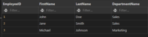
Explaination:
In this example, we define a CTE as “EmployeeDepartments” using the WITH clause. The CTE selects the employee details (EmployeeID, FirstName, LastName) and their corresponding department names (DepartmentName) by joining the “Employees” and “Departments” tables.
Finally, we use the CTE within the main query to directly select the desired columns from the CTE, resulting in a clear and concise syntax.
Recursive Common Table Expression (CTE) in SQL:
- Any technique called a recursive Common Table Expression (CTE) in SQL enables you to query hierarchical data or data with recursive relationships. It aids in the resolution of issues where each row depends on the outcomes of earlier rows returned by the same query. Here is a brief explanation in everyday language:
Consider a table of employees where the columns “EmployeeID” and “ManagerID” indicate which employees report to which managers. You may locate every employee in the reporting chain beginning with a single employee using a recursive CTE.
Example: Suppose, You have this employee data.
EmployeeID | ManagerID
———————-
1 | NULL
2 | 1
3 | 1
4 | 2
5 | 2
You want to find all employees reporting to EmployeeID 1. Here’s a simple recursive CTE to achieve that:
Input:
WITH RecursiveCTE AS (
SELECT EmployeeID, ManagerID
FROM Employees
WHERE EmployeeID = 1 — Starting with EmployeeID 1
UNION ALL
SELECT E.EmployeeID, E.ManagerID
FROM Employees AS E
INNER JOIN RecursiveCTE AS R
ON E.ManagerID = R.EmployeeID
)
SELECT EmployeeID, ManagerID
FROM RecursiveCTE;
Output:
EmployeeID | FirstName | LastName | Salary | SalaryRange
——————————————————-
1 | John | Doe | 50000 | Low
2 | Jane | Smith | 60000 | Medium
3 | Michael | Johnson | 75000 | Medium
4 | Sarah | Brown | 90000 | High
- In this example, we define a recursive CTE named “RecursiveCTE.” We start with the anchor member, which selects EmployeeID 1 from the Employees table.
- Then, we have the recursive member, which joins the Employees table with the RecursiveCTE itself, matching the ManagerID of the current row with the EmployeeID of the previous rows. It continues to add rows until no more matches are found.
- Finally, we select the EmployeeID and ManagerID from the RecursiveCTE, giving us all the employees reporting to EmployeeID 1.
- Recursive CTEs are helpful when dealing with hierarchical data structures like organizational charts or family trees
How to Use a Case WHEN Statement with Multiple Conditions:
The SQL CASE WHEN statement is a conditional expression that enables you to take various actions in response to various situations. It resembles making choices when writing SQL queries.
Explanation:
Consider a database of students that includes the columns “StudentID,” “FirstName,” “LastName,” and “Grade.” You should put pupils into the following categories depending on their grades: “Excellent,” “Good,” “Average,” and “Below Average.” This is made possible via the CASE WHEN statement.
Example:
Let’s say you have the following student data:
StudentID | FirstName | LastName | Grade
—————————————-
1 | John | Doe | 85
2 | Jane | Smith | 75
3 | Michael | Johnson | 92
4 | Sarah | Brown | 65
You want to categorize students based on their grades. Here is a easy example using the CASE WHEN statement:
Input:
SELECT
StudentID,
FirstName,
LastName,
Grade,
CASE
WHEN Grade >= 90 THEN ‘Excellent’
WHEN Grade >= 80 AND Grade < 90 THEN ‘Good’
WHEN Grade >= 70 AND Grade < 80 THEN ‘Average’
ELSE ‘Below Average’
END AS GradeCategory
FROM
Students;
- In this example, the grade category for each student is determined using the CASE WHEN statement within the SELECT statement. This is how it goes:
- The CASE WHEN statement examines each condition individually for each row.
- It labels the GradeCategory column as “Excellent” if the grade is more than or equal to 90.
- The GradeCategory column is given the designation “Good” if the grade falls within the range of 80 and 89 (inclusive).
- The GradeCategory column is given the label “Average” if the grade falls within the range of 70 and 79 (inclusive).
- It labels the GradeCategory column as “Below Average” for any other grade values.
- The outcome will include the original columns (StudentID, FirstName, LastName, Grade), as well as GradeCategory, another column.
Output:
StudentID | FirstName | LastName | Grade | GradeCategory
——————————————————-
1 | John | Doe | 85 | Good
2 | Jane | Smith | 75 | Average
3 | Michael | Johnson | 92 | Excellent
4 | Sarah | Brown | 65 | Below Average
- When doing conditional evaluations and taking different actions in response to particular circumstances, the CASE WHEN statement is helpful. It aids in classifying or transforming data according to logical criteria in your SQL queries.
Using Pivoting and Unpivoting Techniques in SQL:
Pivoting: Using the pivoting and unpivoting techniques in SQL can change the format of data from row-wise to column-wise (pivoting) or from column-wise to row-wise (unpivoting) (unpivoting). Here is a thorough explanation of both ideas with straightforward examples:
Turning rows into columns is known as pivoting. When you wish to rotate or transform data to generate a summary view, it can be helpful. For this, the PIVOT operator is frequently employed. Here’s an Example:
Suppose you have a table named “Sales” with columns “Product,” “Region,” and “Revenue.” The table captures the revenue generated by each product in different regions.
Product | Region | Revenue
————————-
A | East | 1000
A | West | 1500
B | East | 2000
B | West | 1200
You can use the PIVOT operator to pivot the data and display the revenue for each product in separate columns based on the region:
SELECT Product,
[East] AS Revenue_East,
[West] AS Revenue_West
FROM Sales PIVOT (
SUM(Revenue) FOR Region IN ([East], [West])
) AS PivotTable;
The PIVOT operator is used to convert the rows into columns in the aforementioned example. The revenue is determined for each mix of product and area using the SUM(Revenue) aggregation function. This will have the following effects:
Output:
Product | Revenue_East | Revenue_West
————————————-
A | 1000 | 1500
B | 2000 | 1200
Unpivoting:
The process of unpivoting involves changing columns into rows. When normalising or transforming data to do analysis or other activities, it is helpful. Usually, the UNPIVOT operator is employed for this. Here’s an illustration.
Lets take last example: you have a table named “Sales” with columns “Product,” “Revenue_East,” and “Revenue_West.” Each column represents the revenue for a specific product in the respective region.
Product | Revenue_East | Revenue_West
————————————-
A | 1000 | 1500
B | 2000 | 1200
To unpivot the data and display the revenue for each product in different regions in separate rows, you can use the UNPIVOT operator:
SELECT Product,
Region,
Revenue
FROM Sales UNPIVOT (
Revenue FOR Region IN (Revenue_East, Revenue_West)
) AS UnpivotTable;
The UNPIVOT operator is used in the example above to convert the columns into rows. Each time a product and area are combined, a new row is created with the matching revenue. This will have the following effects:
Output:
Product | Region | Revenue
————————-
A | East | 1000
A | West | 1500
B | East | 2000
B | West | 1200
What is SQL View And How Will You Create Them:
- In SQL, Views are a subset of virtual tables. The fields & records (Columns & Rows) of a created view are identical to the database’s actual table. We can create a SQL view by choosing fields/columns from one or more tables from a database. A view may include all table rows or only specific rows according to a set of criteria. This section will teach us how to add, remove, and update Views.
- Example: Create View
- Syntax:
- CREATE VIEW employee_details AS
- SELECT employee_id, employee_name, department
- FROM employees
- WHERE department = ‘IT’;
view named employee_details is created that displays the employee ID, name, and department for employees in the IT department.
See the data in View:
SELECT * FROM employee_details
Create VIEW from multiple tables:
CREATE VIEW MarksView AS
SELECT StudentDetails.NAME, StudentDetails.ADDRESS, StudentMarks.MARKS
FROM StudentDetails, StudentMarks
WHERE StudentDetails.NAME = StudentMarks.NAME;
If you want to see all view tables:
Syntax:
use “database_name”;
show full tables where table_type like “%VIEW”
Stored Procedures in SQL: How to Create it?
SQL-prepared code that has been saved as a stored procedure can be used repeatedly. So, if you frequently develop SQL queries, save them as stored procedures and call them to execute them. Additionally, you may supply parameters to stored procedures in SQL so that they can take action based on the values of the parameters you pass.
- Pre-compiled SQL statements are saved in the database as stored procedures.
- They enable you to combine several SQL statements into a single, repeatable unit.
- Stored procedures can process complex operations, receive input parameters, and return values or result sets.
Steps To Create Stored Procedure in SQL:
Syntax:
CREATE PROCEDURE procedure_name
(parameter1 data_type, parameter2 data_type, …)
AS
BEGIN
— SQL statements to be executed
END
Explanation of the Parameter
- The parameters are the most crucial component. Values are passed to the Procedure using parameters. There are various types of parameters, including the following:
- BEGIN: This is what actually executes, or we could say it is a section that can be executed.
- END: The code will run up until this point.
Execute the procedure
EXEC procedure_name parameter1_value, parameter2_value,
What Are Triggers in SQL and How to Use Them
When a particular event takes place on a table, a SQL trigger is a database object linked to that table that automatically executes a group of SQL queries. Within a database, triggers are used to automate some tasks, ensure data integrity, and enforce business rules. They can be triggered by a variety of actions, such as inserting, updating, or deleting data from a table, and they let you carry out extra actions in response to those actions.
How are SQL triggers implemented?
- SQL triggers are associated with a particular table and defined using SQL statements. The related trigger code is automatically executed when the indicated trigger event (such as an INSERT, UPDATE, or DELETE) takes place on that table. The trigger code may include SQL statements that enforce restrictions, modify data in the same or different tables, or do other actions. Triggers can be set to run before or after the triggering event and are defined to run inside the transaction scope.
What Roles Does SQL Play in Data Science
The Data Life Cycle
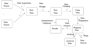
Stages and Operations in the Data Life Cycle:
Data Acquisition/Capture:
Initial step includes obtaining, gathering, or accumulating uncooked statistics from diverse assets.
Data Storage:
Captured records is saved in a structured or unstructured format, regularly accompanied by metadata.
Data Cleaning/Wrangling/Enrichment:
Exploratory Data Analysis (EDA) is carried out to recognize records traits. Metadata validation and augmentation are important. Operations encompass classifying information, visualizing distributions, and handling lacking values.
Data Analysis:
Analyzing the wiped clean and pre-processed statistics the usage of statistical, records mining, or system getting to know strategies.
Data Archival/Preservation:
Results of the analysis are stored, and a choice is made about the destiny of the records.
Data is both purged, archived for destiny use, or published for sharing with different researchers.
Key Operations:
Exploratory Data Analysis (EDA):
Understanding primary records characteristics, classifying datasets, and visualizing distributions.
Data Cleaning:
Handling lacking values, outliers, and replica facts to make sure correctness and completeness.
Data Pre-Processing:
Transformation operations like normalization, scaling, and standardization prepare data for analysis.
Considerations:
Iterative Process:
Analysis may additionally result in in addition questions, requiring extra rounds of information evaluation.
Publication:
Results are often posted with metadata, allowing others to reproduce and reuse the analysis.
Data Disposal:
Careful disposal or archival of statistics, much like coping with valuable assets.
Note:
If desk systems aren’t in a tabular layout, restructuring may be needed earlier than analysis.
Disposal or archival decisions must be made in consideration of the data’s lengthy-term utility.
Loop Diagram:
Indicates the possibility of an iterative process, emphasizing the cyclical nature of statistics analysis.
Data Types Overview:
Two foremost styles of facts: alphanumeric and multimedia.
Multimedia includes audiovisual records (video, pics, audio) encoded in standards like JPEG or MPEG.
Alphanumeric records includes characters representing names or numeric values.
Alphanumeric Datasets:
Alphanumeric datasets, frequently called ‘datasets,’ are collections of statistics objects.
Items are referred to as rows, tuples, statistics, observations, or entities, each describing a actual-global entity with related traits.
Characteristics are attributes, variables, features, or homes, presenting statistics about the entity.
Unified Vocabulary:
The phrases ‘report’ and ‘characteristic’ are used uniformly at some stage in the e book.
Formulas use variables ‘r,’ ‘s,’ ‘r1,’ ‘r2,’ for statistics and ‘A,’ ‘B,’ ‘A1,’ ‘A2,’ for attributes.
Dataset Size and Dimensionality:
Size refers to the range of statistics (cardinality), and dimensionality refers back to the quantity of attributes in a file.
Records may proportion comparable dimensionality, permitting us to discuss the dataset’s dimensionality.
Structured, Semistructured, and Unstructured Datasets:
Datasets are categorized as established (tabular), semistructured, or unstructured.
This e-book by and large specializes in established information, but relational databases can take care of every type.
Record Schema:
The attributes comprising a statistics document are called the schema.
Attributes can be simple (range or label) or complex, with a nested shape.
Complex Attributes:
Complex attributes, like ‘address,’ might also have their personal schema (street number, street deal with, town, zip code, kingdom).
Handling Different Datasets:
Relational databases excel at structured information but can manage semistructured and unstructured statistics.
Table
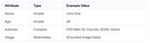
This concise assessment introduces key concepts in facts sorts, datasets, and their type, putting the inspiration for next discussions on facts evaluation.
Types of Datasets
Structured Data:
Datasets where all information proportion a common schema.
Example: new york-flights dataset with attributes like flightid, 12 months, month, and many others.
Can be tabular in layout (CSV files are commonplace), with data prepared into rows and
Columns.
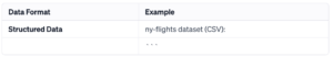
Structured Complex Data:
Some attributes may be complex, containing sub-attributes.
Example: Imaginary worker file with attributes like address and department.
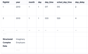
Tabular Data:
Structured records prepared in a table layout.
Each file is normally in a separate line, attributes separated by using a delimiter (e.G., comma).
The first line may additionally comprise the schema names (header).
Semistructured Data:
Records may additionally have unique schemas.
Attributes can be optional, complicated, or have collections of values.
Commonly used for datasets with varying systems.
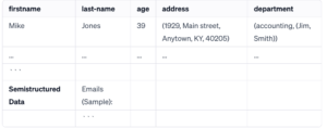
XML and JSON:
Popular formats for semistructured facts.
XML makes use of tags enclosed in angular brackets; JSON makes use of labels, colons, brackets, and curly brackets.
Allows for a hierarchical illustration of complicated attributes.
Graph Data (Semistructured):
Represents objects related to each different (nodes and edges).
Useful for modeling relationships; nodes may additionally have regular attributes.
Directed or undirected, typed or categorised.
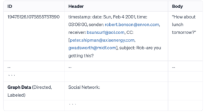
Unstructured Data:
No explicit structure, often refers to text data.
Example: Hate Crime dataset with textual content attributes like Article-Title, Keywords, and Summary.
Requires extra attempt for processing due to lack of express shape.
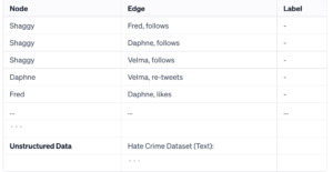
Mix of Formats:
Some datasets are available in a mixture of formats, making them tough for analysis.
Spreadsheets, despite the fact that acting structured, aren’t really dependent because of flexibility in cellular contents.
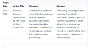
Points:
Different datasets have exclusive structures and formats.
Transformation can be required to evolve facts to the desired layout for analysis.
Spreadsheets and blended-format datasets pose challenges for information analysis.
Types of Domain
Nominal/Categorical Data:
Refers to sets of labels or names.
The area is a finite set without a family members among elements.
No inherent order; ordering is arbitrary.
Examples: ‘Country’ attribute, ‘Type’ attribute in an e mail dataset.
Ordinal Data:
Sets of labels with a linear ordering.
Linear order lets in ranking of values.
Examples: Severity stages of sickness signs, Agreement tiers.
Numerical Data:
Represents quantities and is actually represented by numbers.
Further outstanding into c language and ratio.
Interval: Arbitrary zero; allows assessment and addition/subtraction.
Ratio: Absolute 0; permits ratios and all mathematical manipulations.
Examples: Temperature in Celsius or Fahrenheit (interval), Kelvin (ratio), Time.
Classification of Domains in ny-flights Dataset:
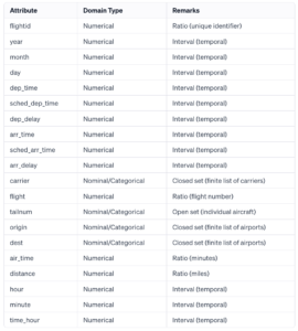
This table represents a simplified dataset with records about flights, which include numerous attributes which includes flight ID, yr, month, departure time, service, flight wide variety, tail wide variety, beginning, vacation spot, airtime, distance, hour, and timestamp.
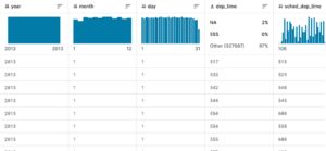
Metadata
Metadata, which is records about records, is crucial for effective records analysis and control. It presents records approximately the traits of the statistics, guiding decisions on operations, cleansing, and preprocessing. Metadata serves several purposes, along with making sure meaningful operations, guiding information cleansing, facilitating reproducibility, and allowing facts sharing.
There are key elements of metadata which are extensively supported:
Structural Metadata: Describes the schema of a dataset and consists of a type of the domain for each attribute.
Domain Metadata: Provides facts approximately the syntactic and semantic components of statistics, along with representations, valid values, and styles.
Provenance/Lineage Metadata: Describes the supply and manipulations applied to facts, assisting to recognize facts origins and ameliorations.
Quality Metadata: Evaluates the fine of statistics, considering factors like accuracy, completeness, consistency, timeliness, and truth.
Key Points:
Metadata aids in significant records operations and guides selections in the course of cleaning and preprocessing.
Provenance metadata is essential for understanding records resources and differences.
Quality metadata assesses factors like accuracy, completeness, consistency, timeliness, and fact.
Metadata ought to be generated ideally at the purchase/storage degree and subtle at some stage in exploratory facts analysis (EDA).
Changes at some stage in cleansing and preprocessing, in addition to evaluation strategies and parameters, ought to be recorded in metadata.
Metadata is important for archiving, enabling data reuse, and making sure accurate know-how of the dataset.
The Role of Databases in the Cycle
- Database Usage Scenarios:
– Data already exists in a database.
– Data is captured and saved in a database due to its size or complexity.
- Options After Accessing Data:
– Export facts to documents for analysis in R, Python, or other software.
– Conduct some paintings (e.G., EDA, facts cleaning) in the database before exporting applicable records.
- Advantages of Database Usage:
– Handling big datasets more efficaciously.
– Strong manipulate get admission to for records protection.
– Managing records evolution and updates efficaciously.
- Considerations for Database Usage:
– Especially beneficial whilst dealing with periodic or updated records.
– Offers advantages even when no longer acting state-of-the-art analysis.
- Challenges with Manual-Intensive Approaches:
– Absence of databases in the method can result in manual-in depth and much less documented consequences.
- Integration with Other Tools:
– Databases may be used along with other tools for coping with data at some point of its existence cycle.
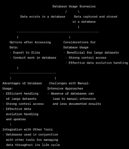
What is Relational Database?
Database and Schema Terminology:
Relational database structures use the term ‘database’ for statistics repositories and ‘schema’ for structure descriptions.
Database Creation:
Start a database server and hook up with it.
Create a database the usage of SQL instructions:
CREATE DATABASE call or CREATE SCHEMA call.
It’s normal to provide descriptive names to databases.
Working with Databases:
After connecting to the server, specify the database to paintings on.
In Postgres: connect database-name
In MySQL: use database-call
Multiple Databases:
Create numerous databases within the identical server, every with a completely unique call.
Users can switch among databases throughout operations.
Table Creation:
After growing a database, the next step is to create tables within that database.
This method is designated and explained in this bankruptcy.
Database and Table Creation Steps:

Database Tables:
Relational databases keep records in tables, considering a database as a set of tables.
Tables are regularly connected, containing associated or linked records.
Creating Tables (SQL):
To create a desk in SQL, use the CREATE TABLE command.
Specify the table name and describe its schema, inclusive of attributes with names and information kinds.
Components of Table Creation:
Components consist of the table name, schema (attributes with names and records types), extension (data in rows), and primary key.
Data Types:
Basic statistics types consist of strings, numbers, and temporal data types. Strings may additionally have various or constant sizes; numbers consist of integers and floats; temporal types cover dates, times, and periods.
Booleans and special sorts for complex information can also be gift.
Example: CREATE TABLE Statement:
Demonstrated with the creation of a desk for the “new york-flights” dataset, specifying attributes and their facts sorts.
Inserting Data:
Use the INSERT INTO statement to feature rows of information to a desk, respecting the schema.
Values ought to in shape the order of attributes within the CREATE TABLE statement.
Inserting Incomplete Data:
NULL marker may be used to indicate missing values whilst placing information.
Destroying a Table:
The DROP TABLE command gets rid of a desk and its data.
Additional Observations:
Tables’ schemas alternate not often, while records in the extension may trade rapidly.
Retrieving schema facts is viable the usage of gadget-particular instructions or queries.
Database Tables:
Relational databases keep information in tables, forming a collection of interconnected tables.
Tables include related or connected facts and are connected thru commonplace attributes.
Table Creation in SQL:
Tables are created the usage of the CREATE TABLE command in SQL.
Example: CREATE TABLE Employees (name char(sixty four), age int, date-of-delivery date, salary float)
Table Components:
Tables have 4 components: call, schema, extension, and number one key.
Each desk need to have a unique call, and the schema defines attributes with names and facts sorts.
Data types consist of strings, numbers, and temporal data kinds.
Data Types in SQL:
Strings constitute sequences of characters, used for nominal/specific attributes.
Numbers consist of integers and floats, representing numerical values with precision considerations.
Temporal information sorts include date, time, timestamp, and c programming language.
Example: CREATE TABLE
Statement for Flights Dataset:
Example: CREATE TABLE NY-FLIGHTS(flightid int, year int, month int, … Time_hour timestamp);
Inserting Data into Tables:
Data is inserted using the INSERT INTO announcement, offering values in the appropriate order or specifying attributes.
Example: INSERT INTO NY-FLIGHTS VALUES(1, 2013, 1, 1, 517, … 2013-01-01 05:00:00);
Handling Incomplete Data:
NULL markers are used to signify lacking values while inserting incomplete facts.
Keys in Tables:
Keys uniquely pick out rows in a desk, frequently composed of a minimum set of attributes.
Primary keys play a critical position, and identifiers (identification) are synthetic keys created for identification purposes.
Creating Ids and Keys:
Ids are often created the use of integers and function primary keys.
Keys can be declared at some stage in desk introduction or brought later the use of ALTER TABLE.
Handling Nulls in Keys:
Primary keys cannot have NULL markers to maintain uniqueness.
What is Data Structure and Its Types:
Data utilized in analytics is regularly supplied in tabular layout, important for Data Mining and Machine Learning algorithms.
Proper desk shape is crucial for evaluation, and the equal information may be prepared in diverse approaches.
Table Formats:
Tables can be wide (unstacked) or narrow (stacked), impacting their comfort for analysis.
Wide tables are favored, with every row describing a distinct document, at the same time as narrow tables may additionally require ameliorations.
Example: Wide vs. Narrow Data:
Example: Wide table with Person as the important thing vs. Narrow desk with (Person, Variable) key.
Transformations can be had to convert narrow statistics into a huge layout appropriate for evaluation.
Untidy Data:
Data may be untidy, as visible in examples with sizes offered as attributes.
Tidy facts follows conventions: values in information cells, attributes inside the schema, each row corresponds to a report.
Data Transformations:
Tidy facts can also require transformations, and R and Python offer tools for managing untidy records.
Examples show the technique of unstacking/pivoting statistics frames to obtain a proper desk shape.
Spreadsheets Issues:
Spreadsheets often introduce issues in records shape, mixing facts and analysis.
Example problems include non-tabular records preparations and issues with margin sums.
Example: Non-Tabular Data in Spreadsheets:
Example of non-tabular statistics in a spreadsheet with statistics spread across rows and columns.
Data shape troubles rise up whilst spreadsheets mix different records types and codecs. Dataset Example: Example of a dataset about worldwide migrants and refugees with troubles including narrow/stacked statistics and hierarchical degrees.
Database Schemas in SQL:
Tabular Data Assumption:
The traditional assumption is that information fits into a tabular format, wherein each document has a nicely-described set of attributes.
Each characteristic has exactly one value in keeping with file.
Common Scenarios for Non-Tabular Data:
Three not unusual situations for records not becoming into a tabular format are heterogeneous records, facts with multi-valued attributes, and complicated facts regarding exclusive but associated occasions or entities.
Heterogeneous Data:
Some records might not be completely homogeneous, sharing commonplace attributes but having variations.
Options for coping with: create a unmarried table with all attributes (the use of NULL for lacking values) or become aware of units of records and create a desk for every.
Multi-valued Attributes:
Some statistics have attributes with a couple of values, leading to the need for a couple of rows to represent the statistics.
Example: Transactional statistics with merchandise associated with transactions.
Complex Data:
Involves eventualities where there are relationships between exclusive information (activities/entities).
Relationships can be one-to-one, one-to-many, or many-to-many.
Foreign keys are used to specific relationships between tables.
Normalization:
Used to cast off redundancy and prevent anomalies within the information.
Example: Breaking down a desk with blended single-valued and multi-valued attributes into separate tables.
Time in Databases:
Time-related facts can upload complexity to the schema.
Example: Storing essential signal measurements over the years for participants in a medical trial.
Database Schema:
A database is a group of related tables.
Schema includes the structure of every desk and overseas keys that link tables.
Data Transformation in SQL:
SQL permits for easy transformation of information, which include normalization and combining tables.
Consideration for Data Analysis:
While most records analysis eventualities choose simple, tabular datasets, databases can take care of extra complex systems whilst wished.
Remember, database design involves a balance among simplicity and the want to accurately represent the actual-global scenario. It calls for a pragmatic approach based totally on the nature of the statistics and the intended use.
Heterogeneous Data:
Some datasets might also have information with optionally available attributes, leading to heterogeneity.
Optional attributes are present below unique occasions, causing some information to lack positive values.
Options for Handling Heterogeneous Data:
Option 1: Create a unmarried table with all possible attributes; use NULL markers for lacking values.
Option 2: Identify homogeneous groups of statistics and create separate tables for every; gets rid of NULL issues.
Example: Optional Attributes in Chicago Employee Dataset:
Chicago employee dataset includes salaried and hourly employees, ensuing in missing values.
A unmarried desk can represent all personnel, using NULLs for lacking values.
Alternatively, cut up the table into two: one for salaried employees and one for hourly employees, heading off lacking values.
Attribute Abbreviations:
Abbreviations used for attributes: Name, Job Title, Department, Full/Part Time (F/P), Salary or Hourly (S/H), Typical Hours (TH), Annual Salary (AS), Hourly Rate (HR).
Flexibility with SQL:
SQL allows combining tables right into a unmarried design or breaking down a single table into a couple of tables primarily based on necessities.
This summary outlines the challenges of coping with heterogeneous records with optional attributes and offers alternatives for addressing them. The Chicago employee dataset example illustrates the alternate-offs between using a single desk with NULLs and developing separate tables for homogeneous groups. SQL provides flexibility for handling these situations.

This representation demonstrates the two options:
- Single table with NULLs and two separate tables for homogeneous groups (hourly and salaried employees).
- Depending on the analysis requirements, either option can be chosen.
Normalization Of Database With Multi-valued Attributes:
Multi-valued Attributes:
Some records in a database may additionally have attributes with multiple values, called multi-valued attributes.
For instance, in a transactional statistics state of affairs, a record may additionally contain a couple of products, each with its own price (e.G., charge).
Single Table Challenges:
In situations with both regular (unmarried-valued) and repeated (multi-valued) attributes, representing information in a unmarried table can cause redundancy and capacity troubles.
Example: Transactional Data:
Transactions regarding more than one products are represented in a single desk with rows for each product.
The key of the table is (Transaction-identification, Product) to ensure strong point for every row.
Issues with Single Table Representation:
Repeating statistics for unmarried-valued attributes (e.G., date, time, keep) may additionally result in anomalies while updating or editing statistics.
Anomalies, like replace anomalies, can bring about inconsistencies in the database.
Normalization Solution:
Normalization includes dividing the data into a couple of tables by separating multi-valued attributes from single-valued attributes.
This method helps take away redundancy and stops anomalies within the database.
Example: Database Design with Normalization:
The transaction records is saved in a single desk with unmarried-valued attributes (Transactions).
Another table stores transaction merchandise, maintaining a connection through the Transaction-id (Products).
Foreign keys (copies of primary keys) are used to maintain connections between tables.
Benefits of Normalization:
Reduces redundancy and minimizes the entire range of cells, optimizing garage.
Enhances information consistency and integrity by way of preventing update anomalies.
SQL for Normalization:
SQL may be used to convert a single table into multiple tables and vice versa, facilitating the normalization system.
Pragmatic Decision for Normalization:
The choice to normalize tables relies upon at the supposed use of information and the information’s inherent structure.
Consideration consists of the threat of anomalies and whether the information might be changed or in most cases analyzed.
Original Single Table
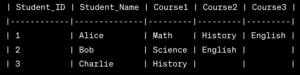
In this table, each row represents a student, and the columns include single-valued attributes (Student_ID, Student_Name) and multi-valued attributes (Course1, Course2, Course3).
Issues:
Redundancy: If a student takes more courses, the identical pupil records is repeated in more than one rows.
Anomalies: Updating or enhancing route information can also cause inconsistencies.
Normalized Table:
Students Table
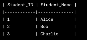
Courses Table:
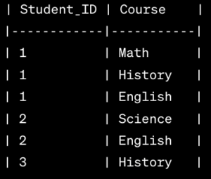
Benefits Of Normalized Table in SQL:
Reduces redundancy:
Student facts is stored once in the Students desk.
Minimizes anomalies:
Updates to course data are less susceptible to inconsistencies.
Foreign Key:
The Student_ID in the Courses table is a overseas key referencing the primary key within the Students desk, preserving the relationship between the two tables.
This normalized structure enhances records integrity and gives a greater flexible and efficient way to control information about students and their guides.
How to Handle Complex Data in Databases
Multi-Valued Attributes:
Records with attributes having several values for a given document are known as multi-valued attributes.
Common in situations in which a report is available in exclusive sizes, each with a corresponding fee.
Resolution includes describing facts the use of several rows, one for every attribute cost.
Transactional Data Example:
In commercial enterprise programs, transactions frequently contain a hard and fast of merchandise/offerings.
Handling transactions with multi-valued attributes (products) may additionally require more than one rows consistent with transaction.
Example: A table for transactions and merchandise, wherein each transaction entails more than one merchandise.
Mixed Situations:
Records might also have both ordinary (single-valued) and repeated (multi-valued) attributes.
Staying inside a single table layout can cause redundancy and capability anomalies.
Normalization:
Used to address redundancy and anomalies in database design.
Involves spreading records into numerous tables by way of separating multi-valued attributes from unmarried-valued ones.
Database Schemas and Normalization Example:
Example of storing transactional information using normalization.
Two tables created: one for transactions (single-valued attributes) and every other for merchandise (multi-valued characteristic).
Primary keys and overseas keys used to maintain relationships between tables.
Types of Relationships in Database:
One-to-One: Each file in a single series is associated with simplest one report in every other series.
One-to-Many: Each record in one collection is associated with one or more records in any other series.
Many-to-Many: Records in a single collection may be associated with numerous information in some other, and vice versa.
Handling Relationships in Tables:
Foreign keys are used to explicit relationships among tables.
One-to-Many: Copy the number one key of the “one” side as a foreign key within the “many” aspect.
Many-to-Many: Create a separate desk with overseas keys from each related tables as its number one key.
Time in Databases:
Temporal data can complicate database schemas.
Example: Recording crucial signs over time in a clinical trial.
Adjusting database shape to house time-associated information.
Database Schema as a Collection of Tables:
A database is a group of related tables, every with its very own schema.
Schemas include primary keys and overseas keys to establish and keep relationships.
Flexibility of Databases:
Databases can handle both easy tabular datasets and extra complicated situations.
Data may be normalized through splitting tables or mixed to create a unmarried desk, as wanted.
Understanding and managing relationships, normalization, and temporal factors are essential in designing effective and flexible databases.
Single-Valued Attributes (Books):
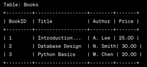
Multi-Valued Attributes (Authors):
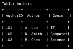
One-to-Many Relationship (Books to Authors):
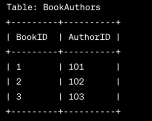
The BookAuthors table establishes a one-to-many courting among books and authors.
Each e book can have a couple of authors, but every author is associated with handiest one book in this example.
Many-to-Many Relationship (Students to Courses):
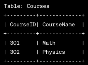
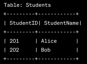
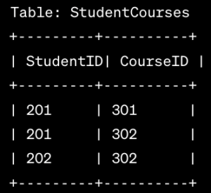
The StudentCourses table establishes a many-to-many courting among students and publications.
Each student can sign up in more than one guides, and each route could have a couple of students.
These examples display the way to shape tables, constitute relationships, and cope with exceptional kinds of attributes in a relational database schema.
Other types of Data in Database
Structured Data and Relational Databases:
Relational databases are designed for based records, regularly organized in tables.
Over time, databases have advanced to deal with semistructured and unstructured facts as well.
XML and JSON Data:
XML and JSON are used for hierarchical or tree-based data.
Hierarchical statistics can be visible as a sequence of 1-to-many relationships forming a tree.
It can be stored in databases both by using flattening it into tables (normalized or unnormalized) or by means of the use of XML/JSON data sorts.
Flattening Hierarchical Data:
Flattening involves breaking hierarchies into degrees, both normalized (a couple of tables) or unnormalized (single desk with repeated statistics).
Example of Hierarchical Data (Biological Classification):
Representation in a flattened desk with attributes for each hierarchy stage.
Splitting the desk into more than one tables to keep away from redundancy.
Handling Hierarchical Relationships:
Unlike tricky eventualities with unbiased one-to-many relationships, hierarchical information with multiple one-to-many relationships does no longer pose issues.
Storing Hierarchical Data, the use of XML/JSON Types:
Modern relational systems permit columns to be declared as XML or JSON sorts.
Data expressed in XML/JSON may be saved without delay in these columns without pulling down.
Example of Storing Hierarchical Data in XML:
XML type column in a table shops hierarchical information.
Data may be loaded into the database without delay and later transformed into a tabular layout for evaluation.
Transformation of XML/JSON to Tabular Format:
Database functions allow changing records from XML/JSON to a flattened desk.
Useful for loading facts in XML/JSON format into the database and then changing it for evaluation, considering equipment that expect tabular information.
These factors summarize the key ideas and examples mentioned in managing hierarchical and semi structured facts in relational databases.
Representation of Graph Data in Relational Databases:
Graph facts may be without difficulty represented using tables: nodes and edges.
The nodes desk represents each node/vertex with shared attributes, and the rims table shops the hyperlinks between nodes.
Nodes and Edges Table Schema in SQL:
nodes table includes attributes which include id, call, and additional functions.
Edges table consists of attributes for the source and destination nodes, along with a non-compulsory label for additional information.
Example of Storing Graph Data as Tables:
CREATE TABLE nodes (
id INTEGER PRIMARY KEY,
name character(16) NOT NULL,
feature1 datatype1,
feature2 datatype2,
…
);
CREATE TABLE edges (
a INTEGER NOT NULL REFERENCES nodes(id) ON UPDATE CASCADE ON DELETE CASCADE,
b INTEGER NOT NULL REFERENCES nodes(id) ON UPDATE CASCADE ON DELETE CASCADE,
label character(256),
PRIMARY KEY (a, b)
);
— Example data insertion
INSERT INTO nodes VALUES (1, ‘Shaggy’, …), (2, ‘Fred’, …), …;
INSERT INTO edges VALUES (1, 2, ‘follows’), (1, 3, ‘follows’), …;
Alternative Approach: Storing Graphs as Matrices:
Use matrices to symbolize graph statistics, in which rows and columns correspond to vertices.
The adjacency matrix has entries indicating the presence or absence of edges between vertices.
Adjacency Matrix Representation:
Boolean adjacency matrix for a simple graph with vertices 1, 2, 3, and four.
Matrix multiplication can reveal records approximately paths in the graph.
Properties of Adjacency Matrices:
Diagonal entries are 0 if there are not any self-loops.
Symmetric for undirected graphs; otherwise, the matrix is directed.
Matrix multiplication offers records about paths and transitive closure.
Graph Analysis within the Database:
While complicated graph algorithms might not be convenient in SQL, simple graph analysis tasks can be done.
Databases are beneficial for storing and managing massive graphs, that can later be analyzed the usage of committed graph gear.
This summary outlines the representation of graph records in relational databases, such as desk schemas, adjacency matrices, and primary graph analysis skills within a database.
How to Export and Import Data in Relational Databases
Text Data in Tables:
Text data in relational databases is often stored using the text data type.
Different databases have varying text types (e.g., text in PostgreSQL, TINYTEXT, TEXT, MEDIUMTEXT, LONGTEXT in MySQL).
Example: Hate Crime Dataset Schema (Postgres):
CREATE TABLE HATE_CRIME(
article_date Date,
article_title char(256),
organization char(128),
city char(64),
state char(2),
url char(32),
keywords Text,
summary Text
);
Inserting Data into Tables:
- Use the INSERT INTO statement to add data to tables.
- Example:
INSERT INTO HATE_CRIME VALUES(
‘3/24/17’,
‘Kentucky Becomes Second State to Add Police to Hate Crimes Law’,
‘Reason’,
‘Washington’,
‘DC’,
‘http://reason.com/blog/2017/03/24/kentucky-becomes-second-state-to-add-pol’,
‘add black blue ciaramella crime delatoba donald gay hate law laws lives louisiana matter police trump add black blue ciaramella crime delatoba donald gay hate law laws lives louisiana matter police trump’,
‘Technically, this is supposed to mean that if somebody intentionally targets a person for a crime because they are police officers, he or she may face enhanced sentences for a conviction. That is how hate crime laws are used in cases when a criminal targets’
);
Importing and Loading Data:
- Use LOAD DATA INFILE (MySQL) or COPY (Postgres) to import data from a file.
- Specify delimiter, enclosed characters, and other options based on the file format.
- Example (MySQL):
LOAD DATA INFILE ‘ny-flights.csv’
INTO TABLE ny_flights
FIELDS TERMINATED BY ‘,’;
ny_flights FROM ‘/path/to/ny-flights.csv’ DELIMITER ‘,’ CSV HEADER;
Updating and Deleting Data:
- Use UPDATE to modify existing data and DELETE to remove data based on specified conditions.
- Example (Update):
UPDATE ny_flights SET flight = ‘8501’ WHERE id = 1;
DELETE FROM ny_flights WHERE origin = ‘JFK’ AND dest = ‘ATL’ AND departure_time BETWEEN ’12:00:00′ AND ’17:00:00′;
Exporting Data:
- Use SELECT INTO OUTFILE (MySQL) or COPY TO (Postgres) to export data to a file.
- Example (MySQL):
SELECT * INTO OUTFILE ‘/path/to/outputfile.csv’ FIELDS TERMINATED BY ‘,’ FROM ny_flights;
Example (Postgres):
COPY ny_flights TO ‘/path/to/outputfile.csv’ DELIMITER ‘,’ CSV HEADER;
Dumping and Restoring Data:
- Use mysqldump (MySQL) or pg_dump (Postgres) to create SQL script backups.
- Example (MySQL):
mysqldump database-name > dump.sql
Example (Postgres):
pg_dump database-name > dump.sql
Restore the backup:
- MySQL: mysql < dump.sql
- Postgres: psql -d new-database-name -f dump.sql
How to Use SQL for Data Cleaning and processing:
The Basic SQL Query:
SQL Foundations:
SQL (Structured Query Language) is essential to running with relational databases.
Basic SQL queries involve SELECT, FROM, and WHERE clauses.
SELECT: Specifies the columns to retrieve.
FROM: Specifies the table(s) from which to retrieve information.
WHERE: Applies situations to clear out the records.
Exploratory Data Analysis (EDA):
Understanding Data:
SQL queries facilitate EDA by means of summarizing, grouping, and aggregating information.
GROUP BY clause helps analyze data primarily based on precise attributes.
Aggregate functions like COUNT, SUM, AVG assist in deriving insights.
Data Cleaning:
Identifying and Handling Missing Data:
SQL queries may be used to pick out missing values (NULL).
UPDATE statements can be employed to update or cope with missing statistics.
Handling Duplicates:
Detect and cast off duplicate facts the use of SQL.
The DISTINCT keyword may be used to retrieve precise statistics.
Correcting Data Types:
Use CAST or CONVERT capabilities to exchange facts sorts.
Ensure consistency in information kinds across columns.
Data Pre-processing:
Normalization:
Normalize statistics to lessen redundancy and dependency.
SQL queries with JOIN operations assist normalize data saved in a couple of tables.
Derived Attributes:
Create new columns with derived attributes the use of SQL expressions.
Example: Calculate age from the birthdate.
Data Transformation:
Use SQL functions for statistics transformation (e.G., UPPER, LOWER, CONCAT).
Ensure uniformity and standardization in textual facts.
Metadata and Implementing Workflows:
Metadata Retrieval:
Extract metadata approximately tables, columns, and constraints using system tables.
Example: Retrieve data from the INFORMATION_SCHEMA in SQL.
Workflow Implementation:
Design and put into effect records processing workflows using SQL.
Create stored procedures or perspectives to encapsulate complicated operations.
Version Control:
Use SQL queries to tune adjustments in facts through the years.
Timestamping facts for versioning and auditing functions.
Integration with Other Tools:
SQL interfaces with diverse information technological know-how tools for seamless integration.
Query outcomes can be further analyzed the usage of statistical equipment like Python or R.
Automation and Scheduling:
SQL queries may be incorporated into automated information cleaning and processing pipelines.
Schedule SQL jobs for periodic data updates and preservation.
What is Data Analysis and How to Get Started with Example:
Purpose of Data Analysis:
Data evaluation entails analyzing, cleaning, transforming, and modeling statistics to discover beneficial facts.
It aids in decision-making, trouble-fixing, and extracting significant insights.
Data Analysis Lifecycle:
Encompasses statistics series, cleaning, exploration, modeling, and interpretation.
Iterative system to refine information and insights.
What Is Data Analysis?
Definition:
Data analysis includes inspecting, cleaning, transforming, and modeling facts to discover useful statistics, draw conclusions, and help decision-making.
Key Components:
Descriptive Statistics: Summarizing and describing main capabilities of a dataset.
Inferential Statistics: Making inferences approximately a population based totally on a pattern of facts.
Supervised Approaches:
Supervised Learning:
Involves training a model on a categorized dataset with enter-output pairs.
Examples include regression and classification algorithms.
SQL is used to prepare and preprocess records for education these fashions.
Unsupervised Approaches:
Unsupervised Learning:
Algorithms perform on unlabelled statistics to discover styles, relationships, or groupings.
Common strategies encompass clustering and dimensionality discount.
SQL aids in data exploration and training for unsupervised algorithms.
Dealing with JSON/XML:
Handling Semi-Structured Data:
JSON (JavaScript Object Notation) and XML (eXtensible Markup Language) are semi-established facts formats.
SQL supports extraction and manipulation of data from JSON and XML systems.
Text Analysis:
Analysing Text Data:
Involves extracting insights from textual facts.
SQL’s string features, pattern matching, and textual content processing skills guide text evaluation.
More on Joins:
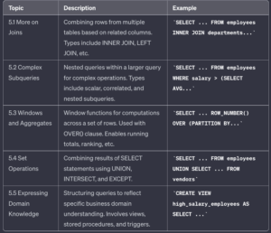
Overview:
This bankruptcy explores extra SQL operators to provide a complete understanding of the language.
Focus on operators not critical to facts evaluation or more advanced standards like WINDOW aggregates.
Understanding Joins:
Joins combine tables primarily based on special situations, producing a end result set.
Joins may be blended with different operations, which includes grouping, aggregation, and choice.
Existential Effect:
When becoming a member of tables, tuples not assembly the be part of situation are dropped, leading to the existential effect.
Illustrated with an instance involving tables EMP(ssn, name, …) and SALES(essn, itemid, amount, date).
Example: Existential Effect (Outer Join):
Query to investigate worker overall performance inside the closing sector may additionally omit employees without a sales.
Solution: Use an outer be a part of (LEFT OUTER JOIN) to keep all personnel, even the ones without sales.
Outer Join Use:
Applied to eventualities in which non-matching tuples are critical, verified with the VAERS and DEATHS tables instance.
Multiplicative Effect:
Occurs when a tuple in one desk fits numerous tuples in every other, ensuing in reproduction rows.
Problematic while the use of aggregates touchy to duplicates.
Complex Subqueries:
Nested Subqueries in FROM Clause:
Use of subqueries within the FROM clause for step-by-step aggregation to avoid multiplicative effects.
Illustrated with a banking scenario concerning branches, loans, and accounts.
Handling Multiplicative Effect:
Caution emphasized in handling multiplicative relationships, ensuring accurate analysis.
Demonstrated solution the use of separate subqueries for loans and bills aggregates before evaluation.
Example: Handling Multiplicative Effect:
Query to locate branches wherein the full loan quantity exceeds total deposits can also produce wrong consequences.
Mastering Complex Subqueries in SQL With Examples:
Introduction to WHERE Clause Subqueries:
SQL widespread lets in complicated situations in the WHERE clause the usage of subqueries.
Different Flavors of WHERE clause subqueries with numerous predicates are explored.
Aggregated Subqueries:
Subqueries with only aggregates in the SELECT clause.
Example: Query to discover employees with a salary better than the average earnings of salaried employees in Chicago.
Subqueries with (NOT) IN:
IN predicate used with a subquery that returns a list of values.
Example: Query to list names and salaries of all managers the use of the IN subquery.
Subqueries with (NOT) EXISTS:
EXISTS predicate exams if a subquery returns a non-empty result.
Example: Query to discover names and salaries of employees in the Research branch if the Marketing department exists.
Subqueries with ANY, ALL:
ANY and ALL predicates evaluate an characteristic to values returned by a subquery.
Example: Query to locate personnel making extra cash than all of us within the Marketing branch.
Subquery Equivalence and Nulls:
Some subquery kinds are redundant and equivalent to others.
Example: Distinction among IN and = ANY, NOT IN and <> ALL, considering the effect of nulls.
Correlated Subqueries:
Subqueries inside the WHERE clause can be correlated, referencing attributes from the outer query.
Example: Query to discover personnel making greater than the average income in their branch.
Optimizing Subqueries:
Discussion on avoiding subqueries when feasible, using opportunity query systems.
Example: Moving subqueries from WHERE to FROM or using joins in place of IN and EXISTS.
SQL Windows and Window Aggregates Functions:
Overview:
Introduction to Windows:
Windows in SQL offer more flexibility than GROUP BY by way of allowing operations on exact units of rows.
Windows aren’t collapsed to a unmarried row, allowing operations inside them.
Window Functions and Syntax:
Window functions appear in SELECT and ORDER BY clauses.
The WINDOW clause syntax includes PARTITION BY, ORDER BY, and FRAME additives.
Components of WINDOW Clause:
PARTITION BY: Creates home windows by using grouping rows with the same values for designated attributes.
ORDER BY: Sorts tuples inside each window, defining row order.
FRAME: Specifies a subset of rows inside each window for aggregate calculations.
Examples: Moving Average Calculation:
SELECT storeid, month, amount, avg(amount) OVER w
FROM Sales
WHERE month BETWEEN 2015/09 AND 2015/12
WINDOW w AS (PARTITION BY storeid, ORDER BY month, ROWS 2 PRECEDING);
Computes the moving average over 3 months for each store.
Multiple Windows in a Query:
SELECT storeid, productid,
sum(amount) OVER everything,
sum(amount) OVER bystore,
sum(amount) OVER byproduct
FROM sales
WINDOW everything AS (),
bystore AS (PARTITION BY storeid),
byproduct AS (PARTITION BY productid);
Computes three different sums using different windows.
Correlated Windows:
SELECT storeid, month, sum(amount) OVER w2a, avg(amount) OVER w2b
FROM sales
WHERE month BETWEEN 2001/09 AND 2001/12
WINDOW w AS (PARTITION BY storeid, ORDER BY month),
w2a AS (w ROWS BETWEEN UNBOUNDED PRECEDING AND CURRENT ROW),
w2b AS (w ROWS BETWEEN 1 PRECEDING AND 1 FOLLOWING);
Computes cumulative sales per month and a cantered average per month.
Advantages and Use Cases:
Fine-grained manage over aggregate calculations inside detailed home windows.
Increased flexibility in comparison to GROUP BY for computing various types of aggregates.
Efficiently handles cumulative, moving, and other complicated mixture calculations.
Extensions: ROLLUP and CUBE
ROLLUP:
Simulates a couple of GROUP BY queries with distinct groupings.
Provides aggregated consequences for various prefix groupings.
CUBE:
Simulates a couple of GROUP BY queries for all viable attribute subsets.
Generates aggregated consequences for diverse combos of grouped attributes.
Summary:
Windows and window aggregates in SQL offer stronger talents for quality-tuned mixture calculations inside exact subsets of facts. The introduction of ROLLUP and CUBE similarly simplifies complicated aggregations and presents green alternatives to standard GROUP BY queries. The flexibility of window functions extends the analytical abilities of SQL, making it a powerful device for data evaluation and reporting.
What are SQL Set Operations and How To Use Them
Overview:
Introduction to Set Operations:
SQL allows set operations, such as UNION, INTERSECT, and EXCEPT.
These operations involve combining the results of queries.
Schema Compatibility:
Tables need to be schema-well matched for set operations.
Schema compatibility method having the identical variety and type of attributes.
Example: UNION Operation
SELECT … FROM … WHERE …
UNION
SELECT … FROM … WHERE …
Example:
SELECT ‘Psychology’ as program, *
FROM PsychologyRank
UNION
SELECT ‘Economy’ as program, *
FROM EconomyRank
UNION
SELECT ‘History’ as program, *
FROM HistoryRank;
Combines rankings of schools in Psychology, Economy, and History.
Example: INTERSECT and EXCEPT Operations
INTERSECT:
SELECT … FROM … WHERE …
INTERSECT
SELECT … FROM … WHERE …
EXCEPT:
SELECT … FROM … WHERE …
EXCEPT
SELECT … FROM … WHERE …
Example (INTERSECT):
SELECT name
FROM PsychologyRank
INTERSECT
SELECT name
FROM EconomyRank;
Retrieves schools that are top ranked in both Psychology and Economy.
Example (Except):
SELECT name
FROM PsychologyRank
EXCEPT
SELECT name
FROM EconomyRank;
Retrieves schools that are top-ranked in Psychology but not in Economy.
Transforming NOT IN with EXCEPT
Example:
SELECT attrA
FROM (SELECT attrB
FROM Table1
EXCEPT
SELECT attrC
FROM Table2) as Temp, Table1
WHERE Temp.attrB = Table1.attrB;
Transforms the NOT IN condition into an EXCEPT operation.
Advantages and Considerations:
Set operations offer powerful methods to mix, examine, and examine information.
Schema compatibility is critical for performing set operations.
Set operations are useful for expressing complex conditions in a concise manner.
Summary:
Set operations in SQL, inclusive of UNION, INTERSECT, and EXCEPT, offer versatile gear for combining and evaluating information from more than one queries. These operations offer concise and expressive approaches to handle diverse analytical eventualities. Additionally, set operations require schema compatibility for significant outcomes. The capacity to convert conditions like NOT IN into equal EXCEPT operations provides to the flexibility and expressiveness of SQL queries.
Expressing Domain Knowledge with CHECK Statements
Overview:
Domain Knowledge in Databases:
Domain knowledge (problem be counted understanding) entails facts and constraints approximately a actual-international area represented inside the statistics.
Benefits of Domain Knowledge:
Facilitates exploratory statistics evaluation (EDA).
Helps become aware of errors, outliers, and lacking values inside the records.
Using CHECK Statements:
The CHECK assertion is used to express constraints on attribute values.
It is employed when developing a desk or added later with ALTER TABLE.
Syntax: CHECK circumstance.
CREATE TABLE NY_FLIGHTS (
flightid int,
year int,
month int CHECK (month BETWEEN 1 and 12),
day int CHECK (day BETWEEN 1 and 31),
dep_time int,
sched_dep_time int,
dep_delay int,
arr_time int,
sched_arr_time int,
arr_delay int,
carrier char(2),
flight char(4),
tailnum char(6),
origin char(3) CHECK (origin IN (‘EWR’, ‘LGA’, ‘JFK’)),
…,
CHECK (sched_dep_time < sched_arr_time)
);
Constraints:
Checks on month, day, and beginning values.
Departure and arrival time constraints.
Exercise five.Thirteen
Additional Constraints in CREATE TABLE:
arr_time have to be later than dep_time and sched_dep_time.
Dep_delay need to be the difference among dep_time and sched_dep_time.
Arr_delay should be the distinction between arr_time and sched_arr_time.
Write a extra complete CREATE TABLE declaration with additional CHECK constraints.
Considerations:
Disabling CHECKs of Data Loading:
Some structures allow disabling checking at some stage in facts loading for overall performance reasons.
This accelerates the loading technique however may additionally permit awful statistics to be inserted.
It’s recommended to let the gadget check data in the course of loading until handling very massive datasets.
Note:
Using CHECK statements in SQL allows the expression of area know-how constraints, helping in fact satisfaction and integrity. These statements are useful for specifying conditions on characteristic values, and making sure that the facts adhere to expectancies. Incorporating area information into the database schema allows effective exploratory records analysis and allows picking out and take care of mistakes within the information. While some structures provide the option to disable checks at some point of data loading for pace, it is typically helpful to permit the device test the information to ensure its integrity.
SQL For Data Science with R
Connecting to a relational database from R entails a systematic system that follows a trendy sample. The number one language for communique with the database is SQL. This phase outlines the simple steps and considerations while running with SQL and R.
Basic Process:
Database Connection:
Establish a connection to the relational database using R.
Common R packages for database interplay consist of RSQLite, RODBC, and DBI.
SQL Queries:
Formulate SQL queries to have interaction with the database.
SQL is used to retrieve, insert, replace, or delete statistics.
Execution and Retrieval:
Execute SQL queries the usage of R capabilities.
Retrieve results into R information structures (e.G., facts frames).
Data Analysis in R:
Analyse and manage the retrieved statistics using R functionalities.
Leverage R’s statistical and visualization capabilities.
Example (R and SQLite):
# Load required package
library(RSQLite)
# Connect to SQLite database
con <- dbConnect(RSQLite::SQLite(), dbname = “your_database.db”)
# Formulate SQL query
query <- “SELECT * FROM your_table;”
# Execute query and fetch data into a data frame
result <- dbGetQuery(con, query)
# Close the database connection
dbDisconnect(con)
# Analyze and visualize data in R
summary(result)
Notes:
Package Choice: The choice of R bundle depends on the specific database system (e.G., SQLite, MySQL, PostgreSQL) and private preference.
SQL Syntax: SQL queries are written in popular SQL syntax within R features. The equal SQL standards apply as in every other context.
Error Handling: Include errors managing to control troubles which includes connection disasters or query mistakes.
SQL For Data Science with Pythonx
Similar to R, connecting Python to a relational database follows a based technique. Python affords various programs for database interplay, and SQL is used because the primary language for conversation.
Basic Process:
Database Connection:
Establish a connection to the relational database using Python.
Common Python applications include sqlite3, psycopg2 (for PostgreSQL), and SQLAlchemy.
SQL Queries:
Formulate SQL queries to have interaction with the database.
Utilize Python’s database interplay capabilities or ORM (Object-Relational Mapping) gear like SQLAlchemy.
Execution and Retrieval:
Execute SQL queries the usage of Python features.
Retrieve and control statistics using Python information structures.
Data Analysis in Python:
Leverage Python’s widespread libraries for data analysis, gadget learning, and visualization.
Example (Python and SQLite):
import sqlite3
# Connect to SQLite database
conn = sqlite3.connect(“your_database.db”)
# Create a cursor object
cursor = conn.cursor()
# Formulate SQL query
query = “SELECT * FROM your_table;”
# Execute query and fetch data
cursor.execute(query)
result = cursor.fetchall()
# Close the database connection
conn.close()
# Analyze and visualize data in Python
print(result)
Notes:
Package Choice: Python gives extraordinary packages primarily based at the database machine. Sqlite3 is used for SQLite, at the same time as different applications like psycopg2 or SQLAlchemy are appropriate for other databases.
SQL Syntax: SQL queries in Python are written as strings and finished the use of suitable capabilities.
Error Handling: Include error managing to address problems like connection issues or query mistakes.
In each R and Python, the fundamental connection and interplay ideas with a relational database remain constant, with SQL serving as the not unusual language for communique. The desire of applications and equipment depends at the database gadget and character choices.