What Is Descriptive Statistics?

Descriptive statistics is a measure used to explain information using numbers, such as mean, median, and mode. Here’s how to calculate it.

The article below will help recognize the differences between descriptive and inferential statistics. We’ll then go through several illustrations of descriptive stats and how to calculate them yourself.

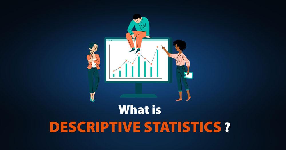
WHAT IS DESCRIPTIVE STATISTICS?

Descriptive Statistics is a statistical method of describing data by specific numbers such as mean or median, mode, and so on. To make it easier for people to be able to comprehend and interpret. They don’t require any generalization or inference beyond what’s available to make it easier to understand and interpret. Descriptive statistics are based on the current information (sample) and not on any mathematical probability theory.

What Is Statistics?

Statistics is collecting and analyzing data to discover percentages (samples) that represent the entire population. In other words, it interprets data to predict the general population.

The two fields of statistics.

• Descriptive Statistics Descriptive Statistics is a statistical measure that provides information about the data.
• Inferential Statistics Inferential Statistics employ inferential statistics when you employ a random sample of data from a group to conclude that population.

Descriptive Statistics vs. Inferential Statistics?

Descriptive statistics provide information through certain numbers, such as mean median, mode, etc., to help comprehend and analyze the data. Descriptive statistics do not require any extrapolation or interpretation beyond the data that is readily available. This means that descriptive statistics are based on the current information (sample) and don’t base themselves on any theories of probability.

Understanding the difference between descriptive statistics and those derived from inferential ones. | Source: The Organic Chemistry Tutor

COMMONLY USED MEASURES

1. Measurement of central tendencies
2. Dispersion measures (or the degree of variability)

What Are the Measures of Central Tendency?

A measure of central tendencies is a single-number data summary usually used to describe data’s centrality. One-number summaries are one of three types.

1. Mean
2. Median
3. Mode

WHAT IS THE MEAN?

Mean is the ratio of that of all observations found in your data to total observations. It is also referred to as the average. So, the term “mean” refers to an integer that is the basis on which the entire information set is distributed.

WHAT IS THE MEDIAN?

The Median is the point that divides the whole of the information into equal parts. One part of the information is lower than the median, while the other portion is more over the median. The Median is determined by organizing the data in ascending or descending order.

• If the total number of observations is unusual, the median is determined in the form of the middle one, in the form of sorted.
• If the numbers of observations are equal, the median is calculated as the median of two middle observations of the format of the sorted form.

Always keep the most important thing in mind the order in which you store information (ascending or ascending) is not a factor in how much the median.

WHAT IS THE MODE?

The number Mode represents the one with the highest frequency within the entire set of data. In other words, the mode represents the value displayed most frequently. Data can be in at least one mode.

• If only one number is displayed most frequently, the data is in one mode, Uni-modal.
• If two numbers are identically displayed frequently, the data can be classified as having two different modes and is referred to as bimodal.
• If greater than two numbers appear often, the data contains more than two possible modes. This is referred to as multi-modal.

Let’s Find the Mean, Median, and Mode

Take a look at the following details:

17, 16, 21, 18, 15, 17, 21, 19, 11, 23

We compute the mean as follows:

To determine the median, we’ll place all the information in an ascending sequence:

11, 15, 16, 17, 17, 18, 19, 21, 21, 23

Because there are ten observations, the total number is even (10). The median is calculated as the median of the two middle observations (fifth and sixth).

The mode is indicated as the number which appears most often. For this data set, 17 and 21 occur twice. This is bi-modal data, with the two modes being 17 and 21.

Some things to keep in mind:

1. Because median and mode do not take into account all data points when making calculations Median and mode are strong against extremes (i.e., they don’t get dependent on outsiders).
2. However, the mean shifts towards the outlier when it considers all data points. If the outlier is large, the mean likely underestimates the information, and if it’s small, then the data is underestimated.
3. If the pattern is symmetrical, the median = mean = mode or what we describe as a “normal distribution.”

What Are Measures of Dispersion?

Measures of Dispersion define the distribution of values around the centre (or the measures of central tendencies).

7 MEASURES OF DISPERSION

1. Absolute deviance from the mean
2. Variance
3. Standard deviation
4. Range
5. Quartiles
6. Skewness
7. Kurtosis

1. ABSOLUTE DEVIATION FROM MEAN

Absolute deviations from mean values, often referred to as Mean Absolute Deviation (MAD), describe the variations within the data set. In an inverse sense, it gives you the absolute average distance for each data element in the set. It’s calculated like this:

• VARIANCE

Variance is a measure of how many data points disperse from the average. A high variance means that the data points are spread wide, while a smaller one indicates that information points lie closer to the data set’s mean. It is calculated as:

• STANDARD DEVIATION

A square root is referred to as”standard deviation. It is calculated as follows:

• RANGE

The range is the gap between this data set’s largest amount and minimum. It can be described as follows:

• QUARTILES

Quartiles refer to the points of the data set which divide it into equal components. Q1 Quartiles Q1, Q2 and Q3 comprise three quartiles: the second, first and quartiles in the set of data.

• 25% of data points are below Q1, while 75% are above.
• 50% of the data points fall below Q2, and 50% are above it. Q2 is nothing more than the median.
• 75% of data points fall below Q3 while 25% exceed it.

• SKEWNESS

The skewness determines the degree of asymmetry in the probability distribution. Skewness could be negative, positive, or undecided. We’ll be focusing on skews that are positive and negative.

• Positive Skew: This happens when the tail on the right-hand side of the curve appears larger than the tail on the left. In these distributions, the mean is larger than that of the mode.
• Negative Skew: This happens in which the left-hand edge of the curvature is larger than the one on the right side. In these cases, the mean is less than the mean.

The most widely employed method for the calculation of Skewness is:

If the skewness of the distribution is zero and the distribution is symmetrical, it’s. If it’s negative, the distribution is skewed negatively, and if the skewness is positive, it’s positively tilted.

Three instances of Skewness. | Image: Wikipedia

• KURTOSIS

Kurtosis indicates that the information is either light-tailed (lack in extremes) or heavy-tailed (outliers are present) compared with normal distribution. There are three types of kurtosis.

Three forms of Kurtosis. | Image: Wikipedia

• Mesokurtic The situation where the kurtosis is zero is similar to normal distributions.
• Leptokurtic occurs when you see the tail of your distribution very heavy (outlier in the present), and kurtosis is more than the normal distribution.
• The term “Platykurtic” refers to the condition that occurs when The term “Platykurtic” occurs where the tail is very light (no outlier). The kurtosis is less than the normal distribution.