
What is Feature Selection?
Feature selection refers to selecting relevant features or variables from a more extensive set in a dataset, aiming to improve accuracy and efficiency by eliminating irrelevant, redundant, or noisy elements that negatively impact machine-learning models.
Feature selection methods should be selected based on the specific problem at hand and the dataset’s characteristics, considering both overfitting, model interpretability, and computational complexity issues. When used properly, feature selection can reduce overfitting while improving model interpretability and decreasing models’ computational complexity.
You may also like to read: Everything You Need To Know About Feature Selection
Why Feature Selection?
Feature selection aims to reduce data dimensionality and optimize machine learning models’ performance.
There are various reasons for selecting features:
- Improved accuracy: By selecting only relevant features, machine learning models can achieve increased accuracy and lower overfitting risk.
- Faster Training and Inference: By decreasing the number of features, training time and making predictions can be significantly decreased; this feature reduction approach is especially advantageous in real-time applications.
- Better Interpretability: By decreasing the number of features, interpretation becomes simpler and it becomes simpler to comprehend how features relate to target variables.
- Reduced data storage and processing requirements: By choosing only relevant features for storage and processing purposes, selectinging subsets reduces the amount of information which needs to be stored and processed – this can be especially valuable where limited resources exist for data storage and processing needs.
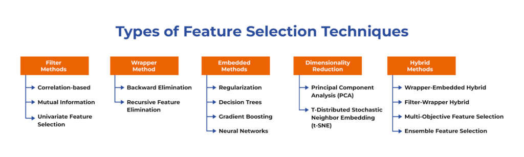
Types of Feature Selection Techniques
Several feature selection techniques can be used in machine learning:
Filter Methods
Filter methods in feature selection is a technique for selecting features based on specific statistical properties such as correlation or mutual information. As it operates independent from machine learning algorithms and doesn’t involve training the model, this makes the filter method a fast and efficient method to select relevant features from datasets.
Different types of filter methods can be used for feature selection:
Correlation-based
This method utilizes correlation coefficients between features and target variables to assess their relevance; those with higher correlation coefficients will be considered more pertinent and considered for inclusion into a model.
Here is an example of performing correlation-based feature selection using Python:
import pandas as pd
import numpy as np
import seaborn as sns
import matplotlib.pyplot as plt

# load the dataset
data = pd.read_csv('data.csv')

# create a correlation matrix
corr_matrix = data.corr().abs()

# create a heatmap
sns.heatmap(corr_matrix, cmap='YlGnBu')
plt.show()

# set a threshold for correlation coefficients
threshold = 0.7

# create a mask to ignore self-correlation and duplicate values
mask = np.triu(np.ones_like(corr_matrix, dtype=bool))

# create a new correlation matrix with only highly correlated features
high_corr_features = corr_matrix.mask(mask).stack().reset_index().rename(columns={0: 'correlation', 'level_0': 'feature1', 'level_1': 'feature2'})
high_corr_features = high_corr_features[high_corr_features['correlation'] > threshold]

# drop one of the correlated features
for i in range(len(high_corr_features)):
    feature1 = high_corr_features.iloc[i]['feature1']
    feature2 = high_corr_features.iloc[i]['feature2']
    if feature1 in data.columns and feature2 in data.columns:
        if corr_matrix.loc[feature1, feature2] > corr_matrix.loc[feature2, feature1]:
            data.drop(feature1, axis=1, inplace=True)
        else:
            data.drop(feature2, axis=1, inplace=True)

# print the remaining features
print(data.columns)
Chi-Squared Test
This method establishes an indicator of independence between features and target variables. Only features that show high degrees of separation from their target variable will be chosen as candidates for inclusion into a model.
Here is an example of using the Chi-Squared test in Python for feature selection:
import pandas as pd
from sklearn.feature_selection import SelectKBest
from sklearn.feature_selection import chi2

# load the data
data = pd.read_csv('data.csv')

# separate the features and target variable
X = data.iloc[:, :-1]
y = data.iloc[:, -1]

# apply SelectKBest class to extract top 10 best features
best_features = SelectKBest(score_func=chi2, k=10)
fit = best_features.fit(X, y)

# summarize scores for each feature
scores = pd.DataFrame({'Feature': X.columns, 'Score': fit.scores_})
scores = scores.sort_values('Score', ascending=False)

# print the top 10 features
print(scores.head(10))
Mutual Information
This method measures the mutual dependency between features and target variables, and selects features with high mutual information as more suitable candidates for use in modeling.
Here is an example code in Python for performing mutual information-based feature selection using scikit-learn’s SelectBest method:
from sklearn.datasets import load_iris
from sklearn.feature_selection import SelectKBest, mutual_info_classif

# load the iris dataset
iris = load_iris()
X = iris.data
y = iris.target

# select the top 2 features using mutual information
k = 2
selector = SelectKBest(mutual_info_classif, k=k)
X_new = selector.fit_transform(X, y)

# print the selected features
mask = selector.get_support()  # mask of selected features
selected_features = iris.feature_names[mask]
print(selected_features)
Variance Threshold
This method removes features with low variance that do not contribute significantly to model performance, in the assumption that they do not significantly contribute.
Here is an example of Variance Threshold feature selection using Python’s scikit-learn library:
from sklearn.feature_selection import VarianceThreshold
import numpy as np

# create a sample dataset with 3 features
X = np.array([[0, 1, 0], [0, 1, 1], [1, 0, 0], [0, 1, 1], [0, 0, 0]])

# initialize a VarianceThreshold object with a threshold of 0.2
selector = VarianceThreshold(threshold=0.2)

# fit the selector to the data
selector.fit(X)

# transform the data to remove low-variance features
X_new = selector.transform(X)

# print the selected features
print(X_new)
Univariate Feature Selection
This method involves selecting features based on their significance to a target variable, using statistical tests like F-test or Chi-squared test to select those most pertinent features.
Here’s an example of performing univariate feature selection using SelectKBest and f_classif in Python:
import pandas as pd
from sklearn.feature_selection import SelectKBest, f_classif

# load data
data = pd.read_csv("data.csv")
X = data.drop("target", axis=1)
y = data["target"]

# feature selection
k_best = SelectKBest(score_func=f_classif, k=5) # select top 5 features
X_best = k_best.fit_transform(X, y)
the machine learning pipeline, as it can significantly impact a model’s accuracy and generalization performancae. In addition, a well-designed feature engineering process can also reduce the risk of overfitting and improve the interpretability of the model.
Wrapper Method
Wrapper methods in feature selection represent a family of methods that use machine learning models to evaluate different subsets of features, then use search algorithms to explore possible feature subsets until finding one which maximizes model performance.
The three main types of wrapper methods are:
Forward Selection
Forward Selection method begins with an empty feature set and incrementally adds one feature at a time until no further enhancements would improve its performance. Next, model evaluation occurs for every subset added until there are none left that produce optimal performance; then, this process continues until all available enhancements have been found for inclusion into the set.
Here is an example of forward selection using Python:
First, let’s import the necessary libraries:
codeimport pandas as pd
from sklearn.feature_selection import SequentialFeatureSelector
from sklearn.linear_model import LinearRegression
Next, let’s load a sample dataset. For this example, we’ll use the Boston Housing dataset from scikit-learn
codefrom sklearn.datasets import load_boston
boston = load_boston()
X = pd.DataFrame(boston.data, columns=boston.feature_names)
y = pd.Series(boston.target, name='target')
Scikit-learn provides us with an efficient method for performing forward selection using SequentialFeatureSelector class; here, a linear regression model serves as our estimator:
codeestimator = LinearRegression()
selector = SequentialFeatureSelector(estimator, n_features_to_select=5, direction='forward')
selector.fit(X, y)
In this example, we specify that we want to select 5 features (n_features_to_select=5) using forward selection (direction=’forward’). In doing this, the fit method of our selector object will perform forward selection to identify and select only 5 best features from among all those eligible for selection.
Now we can access our list of selected features:
codeselected_features = X.columns[selector.get_support()]
print(selected_features)
This will print the names of the 5 selected features.
Backward Elimination
This method starts with all features and removes one feature at a time until the model’s performance is no longer improved. This process continues until no additional features can be removed.
Here’s an example of how to perform backward elimination using sklearn and statsmodels libraries in Python:
import pandas as pd
import numpy as np
import statsmodels.api as sm
from sklearn.linear_model import LinearRegression

# load dataset
data = pd.read_csv("dataset.csv")

# separate dependent and independent variables
X = data.iloc[:, :-1].values
y = data.iloc[:, -1].values

# add a column of ones to X (required for statsmodels library)
X = np.append(arr = np.ones((len(X), 1)), values = X, axis = 1)

# create a list of column names
cols = list(data.columns)

# set the significance level
SL = 0.05

# fit the full model using OLS (Ordinary Least Squares) method
regressor_OLS = sm.OLS(endog = y, exog = X).fit()

# start backward elimination
while True:
    # find the predictor with the highest p-value
    max_pvalue = max(regressor_OLS.pvalues).astype(float)
    if max_pvalue > SL:
        # remove the predictor with the highest p-value
        idx = np.argmax(regressor_OLS.pvalues)
        X = np.delete(X, idx, 1)
        cols.pop(idx)
        # refit the model without the removed predictor
        regressor_OLS = sm.OLS(endog = y, exog = X).fit()
    else:
        break

# print the selected features
print(cols)
Recursive Feature Elimination
This method starts with all features and trains the model, then removes the least important feature and repeats the process until a desired number of features is reached or the model’s performance is no longer improved.
Here is an example of using Recursive Feature Elimination (RFE) for feature selection in Python:
from sklearn.feature_selection import RFE
from sklearn.linear_model import LinearRegression
from sklearn.datasets import load_boston

# Load the Boston Housing dataset
boston = load_boston()

# Define the predictor and target variables
X = boston.data
y = boston.target

# Create a Linear Regression model
lr = LinearRegression()

# Create an RFE object to select top 5 features
rfe = RFE(lr, n_features_to_select=5)

# Fit the RFE object to the data
rfe.fit(X, y)

# Print the ranking of each feature
print(rfe.ranking_)

# Print the selected features
print(boston.feature_names[rfe.support_])
Embedded Methods
Embedded methods are feature selection techniques used during model training to identify relevant features more quickly, eliminating the need for separate feature selection steps. These methods aim to find and select those most important to model training without disrupting its process too much.
There are various embedded methods used in feature selection, including:
Regularization
This method adds a penalty term to a model’s objective function in order to reduce coefficients associated with less significant features towards zero and create a model which only includes key aspects.
Here’s an example of Lasso regularization being applied in Scikit-Learn library as feature selection technique:
from sklearn.linear_model import Lasso
from sklearn.datasets import load_boston
from sklearn.preprocessing import StandardScaler
from sklearn.model_selection import train_test_split

# Load dataset
boston = load_boston()

# Split data into training and testing sets
X_train, X_test, y_train, y_test = train_test_split(boston.data, boston.target, test_size=0.3, random_state=42)

# Scale features to have zero mean and unit variance
scaler = StandardScaler()
X_train = scaler.fit_transform(X_train)
X_test = scaler.transform(X_test)

# Create Lasso model for feature selection
lasso = Lasso(alpha=0.1)
lasso.fit(X_train, y_train)

# Get coefficients of the features
coef = lasso.coef_

# Print coefficients of the features
for feature, coef in zip(boston.feature_names, coef):
    print(feature, ':', coef)
Decision Trees
Decision trees are an algorithm designed to select relevant features from large amounts of data. By splitting up each node into its most essential features, a decision tree reveals all relevant traits in an image-like display, making feature selection simpler.
Here is an example of using decision trees embedded method in Python for performing feature selection:
from sklearn.datasets import make_classification
from sklearn.tree import DecisionTreeClassifier
from sklearn.model_selection import train_test_split
from sklearn.metrics import accuracy_score
import matplotlib.pyplot as plt

# generate synthetic dataset
X, y = make_classification(n_samples=1000, n_features=20, n_informative=5, n_redundant=0, random_state=42)

# split data into train and test sets
X_train, X_test, y_train, y_test = train_test_split(X, y, test_size=0.3, random_state=42)

# create decision tree classifier
clf = DecisionTreeClassifier(random_state=42)

# fit the classifier on training data
clf.fit(X_train, y_train)

# evaluate the model on test data
y_pred = clf.predict(X_test)
acc = accuracy_score(y_test, y_pred)
print("Accuracy before feature selection:", acc)

# plot feature importances
importances = clf.feature_importances_
indices = sorted(range(len(importances)), key=lambda k: importances[k], reverse=True)
plt.bar(range(X.shape[1]), importances[indices])
plt.xticks(range(X.shape[1]), indices)
plt.title("Feature Importances")
plt.show()

# perform feature selection using decision trees embedded method
from sklearn.feature_selection import SelectFromModel

# specify the threshold for feature selection
threshold = 0.05

# create feature selector object
selector = SelectFromModel(clf, threshold=threshold, prefit=True)

# apply feature selection on training data
X_train_selected = selector.transform(X_train)

# fit the classifier on selected features
clf.fit(X_train_selected, y_train)

# apply feature selection on test data
X_test_selected = selector.transform(X_test)

# evaluate the model on selected features
y_pred_selected = clf.predict(X_test_selected)
acc_selected = accuracy_score(y_test, y_pred_selected)
print("Accuracy after feature selection:", acc_selected)
Gradient Boosting
Gradient boosting is an ensemble method which involves building multiple weak models and then combining them together to produce one stronger model. It uses an algorithm to identify key features while weaker models are trained on subsets of data which focus specifically on these features.
Here is an example of using Gradient Boosting with Python and Scikit-learn for feature selection:
from sklearn.ensemble import GradientBoostingClassifier
from sklearn.datasets import make_classification
from sklearn.feature_selection import SelectFromModel

# Generate a random dataset
X, y = make_classification(n_samples=1000, n_features=20, n_informative=5, n_redundant=5, random_state=42)

# Fit a Gradient Boosting model to the data
gb = GradientBoostingClassifier(random_state=42)
gb.fit(X, y)

# Select features based on importance scores from the model
sfm = SelectFromModel(gb, threshold=0.1)
X_new = sfm.fit_transform(X, y)

# Print the selected feature indices
print(sfm.get_support(indices=True))
In this example, we begin by creating a random dataset consisting of 20 features and 1000 samples using scikit-learn’s make_classification function and then fitting a Gradient Boosting model using its GradientBoostingClassifier class.
After this step, we use the SelectFromModel class to identify features with significance scores greater than or equal to 0.1 and create a transformed feature matrix X_new that contains only these selected features. Finally, using get_support method we print their indices.
Neural Networks
Neural networks can be effectively leveraged as feature selection tools by adding regularization terms or dropout layers into their model architecture. Such techniques help eliminate less essential features to maximize model performance and eliminate those which don’t belong.
Here is an example of using Keras in Python for feature selection with neural networks:
import pandas as pd
from sklearn.model_selection import train_test_split
from sklearn.preprocessing import StandardScaler
from keras.models import Sequential
from keras.layers import Dense

# load data
data = pd.read_csv('data.csv')

# separate features and target
X = data.drop('target', axis=1)
y = data['target']

# split data into training and testing sets
X_train, X_test, y_train, y_test = train_test_split(X, y, test_size=0.2, random_state=42)

# standardize features
scaler = StandardScaler()
X_train = scaler.fit_transform(X_train)
X_test = scaler.transform(X_test)

# define model
model = Sequential()
model.add(Dense(64, activation='relu', input_shape=(X_train.shape[1],)))
model.add(Dense(1, activation='sigmoid'))

# compile model
model.compile(loss='binary_crossentropy', optimizer='adam', metrics=['accuracy'])

# train model
model.fit(X_train, y_train, epochs=50, batch_size=32, validation_data=(X_test, y_test), verbose=0)

# get feature weights from trained model
weights = model.get_weights()[0]

# create dataframe of features and weights
feat_weights = pd.DataFrame({'feature': X.columns, 'weight': abs(weights).mean(axis=1)})

# sort by feature weight
feat_weights = feat_weights.sort_values('weight', ascending=False)

# print top 10 features
print(feat_weights.head(10))
Before loading our data into an R environment for processing, we first separate its features from its target variable and standardize using StandardScaler. Then, after creating our neural network model in Keras with binary cross entropy loss and Adam optimizer settings and training on training data sets, respectively, our model can be run again with testing data sets as an evaluation stage.
When our model is trained, we use the get_weights() method to obtain its weights. After we take their absolute value and calculate their mean value per feature weights, we create a dataframe with features sorted in descending order by weights for sorting purposes.
Dimensionality Reduction
Dimensionality reduction is a technique designed to decrease the number of features within a dataset by mapping it onto lower-dimensional space, to simplify while still providing important data insights. It helps machine learning models avoid overfitting by simplifying data while keeping key insights intact decreasing overfitting and computational complexity.
There are two primary techniques used for dimensionality reduction:
Principal Component Analysis (PCA)
This technique converts data to principal components – linear combinations of original features that capture significant variation – for analysis. Selecting how many principal components is up to you; either setting threshold variance thresholds or using cross-validation techniques may help.
Here’s an example of using Principal Component Analysis (PCA) in Python for feature selection to reduce overfitting and computational complexity in machine learning models. This technique may reduce overfitting while simultaneously decreasing computational burden.
There are two primary methods for dimensionality reduction techniques.
from sklearn.decomposition import PCA
from sklearn.datasets import load_breast_cancer
import pandas as pd

# load breast cancer dataset
data = load_breast_cancer()
df = pd.DataFrame(data.data, columns=data.feature_names)

# normalize the data
df_norm = (df - df.mean()) / df.std()

# perform PCA
pca = PCA(n_components=5)
pca.fit(df_norm)
df_pca = pca.transform(df_norm)

# create a new dataframe with the selected features
df_selected = pd.DataFrame(df_pca, columns=['PC1', 'PC2', 'PC3', 'PC4', 'PC5'])

# print explained variance ratio
print('Explained variance ratio:', pca.explained_variance_ratio_)
T-Distributed Stochastic Neighbor Embedding (t-SNE)
This technique for visualizing high-dimensional data in two or three dimensions uses subspace nearerness estimation (t-SNE) mapping each data point onto its new subspace while maintaining similarity among them. t-SNE can help visualize complex datasets.
Here is an example of using the t-SNE algorithm in Python for feature selection:
import numpy as np
import pandas as pd
from sklearn.manifold import TSNE

# Load data
data = pd.read_csv('data.csv')

# Separate features and target variable
X = data.drop('target', axis=1)
y = data['target']

# Create t-SNE object
tsne = TSNE(n_components=2, random_state=42)

# Fit and transform data
X_tsne = tsne.fit_transform(X)

# Calculate feature importance
feature_importance = np.abs(tsne.embedding_).sum(axis=0)

# Print feature importance scores
for i, score in enumerate(feature_importance):
    print(f'Feature {i}: {score:.2f}')
At first, we load and separate features from a target variable before creating a two component t-SNE object to fit and transform data. Next we calculate feature importance scores by adding up absolute values of embedded t-SNE embedding for every feature and finally printing off those scores for every attribute.
Note that t-SNE is typically employed only as an aid for data visualization; it cannot be relied upon to select features; rather it serves primarily to distinguish among groups of data points and help select those most important to distinguishing among them.
Hybrid Methods
Hybrid methods combine multiple feature selection techniques in order to optimize their performance, often making these approaches more efficient than using just one method alone. Here are some commonly-used hybrid approaches:
Wrapper-Embedded Hybrid
This method combines the benefits of both wrapper and embedded methods. After applying an embedded method to narrow down its feature space, a wrapper method then searches for an optimal subset of features.
Here’s an example of using Recursive Feature Elimination with Cross Validation (RFECV), an embedded hybrid method wrapper method in Python for feature selection:
from sklearn.datasets import make_friedman1
from sklearn.feature_selection import RFECV
from sklearn.linear_model import LinearRegression

# generate some sample data
X, y = make_friedman1(n_samples=200, n_features=30, random_state=0)

# initialize a linear regression model
model = LinearRegression()

# initialize the RFECV algorithm
rfecv = RFECV(estimator=model, step=1, cv=5)

# fit the RFECV algorithm on the data
rfecv.fit(X, y)

# print the selected features
print("Selected Features: ", rfecv.support_)
Filter-Wrapper Hybrid
This method combines the strengths of filter and wrapper methods. First it uses filter methods to select features based on performance; then uses wrapper methods to search for optimal subset of features.
Here is an example of using SelectKBest and RandomForestClassifier in Python to implement Filter-Wrapper hybrid feature selection:
from sklearn.datasets import load_iris
from sklearn.ensemble import RandomForestClassifier
from sklearn.feature_selection import SelectKBest, f_classif
from sklearn.model_selection import train_test_split
from sklearn.metrics import accuracy_score

# Load the iris dataset
iris = load_iris()

# Split the dataset into train and test sets
X_train, X_test, y_train, y_test = train_test_split(iris.data, iris.target, test_size=0.3, random_state=42)

# Apply feature selection using SelectKBest and f_classif
selector = SelectKBest(score_func=f_classif, k=2)
X_train_new = selector.fit_transform(X_train, y_train)
X_test_new = selector.transform(X_test)

# Train a random forest classifier on the selected features
clf = RandomForestClassifier(n_estimators=100, random_state=42)
clf.fit(X_train_new, y_train)

# Predict the class labels for test set
y_pred = clf.predict(X_test_new)

# Evaluate the performance of the classifier
acc = accuracy_score(y_test, y_pred)
print("Accuracy:", acc)
Multi-Objective Feature Selection
This method takes multiple criteria into account when choosing features, including accuracy and complexity, in order to select an optimum subset that strikes an equilibrium between these criteria.
Here is an example in Python using the PyGMO library for multi-objective feature selection:
import numpy as np
from sklearn.datasets import make_classification
from sklearn.model_selection import train_test_split
from sklearn.metrics import accuracy_score
from pygmo import hypervolume, non_dominated_front_2d, fast_non_dominated_sorting

# Generate random data
X, y = make_classification(n_samples=1000, n_features=10, n_informative=5, random_state=42)

# Split data into train and test sets
X_train, X_test, y_train, y_test = train_test_split(X, y, test_size=0.2, random_state=42)

# Define the fitness function to be maximized
def fitness_function(features):
    # Extract the selected features
    selected_features = X_train[:, features]

    # Train a classifier
    clf = DecisionTreeClassifier(random_state=42)
    clf.fit(selected_features, y_train)

    # Evaluate the classifier on the test set
    y_pred = clf.predict(X_test)
    accuracy = accuracy_score(y_test, y_pred)

    # Compute the complexity of the selected features
    complexity = len(features)

    # Return the fitness values as a tuple
    return (accuracy, -complexity)

# Define the optimization problem
class FeatureSelectionProblem:
    def __init__(self, num_features):
        self.num_features = num_features

    def fitness(self, x):
        return fitness_function(x)

    def get_bounds(self):
        return ([0] * self.num_features, [1] * self.num_features)

    def get_name(self):
        return "Feature Selection"

# Create the PyGMO algorithm object
algo = pg.algorithm(pg.nsga2(gen=1000))

# Create the PyGMO problem object
problem = pg.problem(FeatureSelectionProblem(num_features=10))

# Run the optimization
pop = algo.evolve(population_size=100, problem=problem)

# Extract the non-dominated solutions
fronts = non_dominated_front_2d(pop.get_f())
non_dominated_solutions = [pop.get_x()[i] for i in fronts[0]]

# Print the non-dominated solutions
for solution in non_dominated_solutions:
    selected_features = [i for i, x in enumerate(solution) if x == 1]
    accuracy, complexity = fitness_function(selected_features)
    print("Accuracy: {:.4f}, Complexity: {}".format(accuracy, complexity))

# Compute and print the hypervolume indicator
hv = hypervolume(pop.get_f())
print("Hypervolume: {:.4f}".format(hv))
This example employs the NSGA-II algorithm to optimize accuracy and complexity in a decision tree classifier. A fitness function is used to assess the accuracy and complexity of features selected from the training set using a decision tree classifier. A class called FeatureSelectionProblem wraps this fitness function while providing problem bounds to PyGMO via PyEVO’s evolve method; non-dominated solutions extracted using non_dominated_front_2d function is then extracted while hypervolume indicator computed with hypervolume function.
Ensemble Feature Selection
This method utilizes multiple feature selection techniques and combines their results in order to select only those features which are most important, providing increased stability and robustness of feature selection.
Here’s an example of ensemble feature selection using Python:
from sklearn.datasets import make_classification
from sklearn.feature_selection import SelectKBest, chi2, f_classif, RFE
from sklearn.ensemble import RandomForestClassifier
from mlxtend.feature_selection import SequentialFeatureSelector
from sklearn.pipeline import Pipeline
from sklearn.model_selection import cross_val_score
from sklearn.metrics import accuracy_score

# Generate some random data for demonstration
X, y = make_classification(n_samples=100, n_features=20, n_informative=10, n_redundant=5, random_state=42)

# Define the individual feature selection methods
skb = SelectKBest(score_func=f_classif, k=5)
rfe = RFE(estimator=RandomForestClassifier(), n_features_to_select=5)
sfs = SequentialFeatureSelector(estimator=RandomForestClassifier(), k_features=5, forward=True, scoring='accuracy', cv=5)

# Define the ensemble feature selection pipeline
ensemble_pipeline = Pipeline([
    ('fss', ('passthrough')),
    ('clf', RandomForestClassifier(random_state=42))
])

# Evaluate the performance of individual feature selection methods and the ensemble feature selection method
scores = []
for name, feature_selector in [('Univariate', skb), ('Recursive', rfe), ('Sequential', sfs), ('Ensemble', ensemble_pipeline)]:
    if name != 'Ensemble':
        X_selected = feature_selector.fit_transform(X, y)
        clf = RandomForestClassifier(random_state=42)
        score = cross_val_score(clf, X_selected, y, cv=5, scoring='accuracy').mean()
    else:
        # Define the feature selection pipeline with ensemble method as the final estimator
        ensemble_pipeline.steps[0] = ('fss', feature_selector)
        score = cross_val_score(ensemble_pipeline, X, y, cv=5, scoring='accuracy').mean()
    scores.append(score)

# Print the performance scores
for name, score in zip(['Univariate', 'Recursive', 'Sequential', 'Ensemble'], scores):
    print(f'{name} feature selection accuracy: {score:.3f}')
How to Choose a Feature Selection Model?
Selecting an effective feature selection model depends on several variables, including dataset type and size, problem nature, available computational resources, and desired level of accuracy. However, here are some general guidelines that should help when making this selection:
Before choosing a feature selection model, it is important to comprehend your data and problem thoroughly. Take time to carefully consider all features relating to target variables and any relationships they might share between each feature type and target variables.
- Select an Appropriate Model Type: Determine an optimal feature selection model type by considering its characteristics; for example, wrapper methods might work better if the data has many features. Filter methods could prove more suitable if there’s noise in your data set.
- Evaluate Model Performance: Evaluate your feature selection model on an evaluation or holdout dataset using accuracy, precision, recall and other metrics to gauge its efficacy.
- Consider computational resources: Some feature selection methods require significant computational resources; consider available resources, like processing power and memory space, when choosing an approach that best meets those requirements.
- Comparing with Other Models: When choosing a model for use, always compare its performance against competing ones to ensure it provides optimal solutions to data and problems.
Feature Selection in Python
Several libraries in Python can be used for feature selection, including Scikit-learn, XGBoost, and LightGBM. Here is an example of performing feature selection using Scikit-learn:
Import the necessary libraries:
from sklearn.datasets import load_breast_cancer

from sklearn.feature_selection import SelectKBest

from sklearn.feature_selection import f_classif
Load the dataset:
data = load_breast_cancer()

X = data.data

y = data.target
Apply the feature selection method:
# Select the 10 best features based on the f_classif score

selector = SelectKBest(score_func=f_classif, k=10)

X_new = selector.fit_transform(X, y)
Print the selected features:
# Print selected feature names
mask = selector.get_support() # list of booleans
new_features = [] # The list of your K best features
for bool, feature in zip(mask, data.feature_names):
    if bool:
        new_features.append(feature)
print(new_features)
This will generate the indices of 10 features selected. We utilized the f_classif score function, which measures ANOVA F-value between each feature and target variable, along with setting k = 10 to select only these 10 features. You may experiment with other score functions or setting different k values to observe how they impact selected features.
Methods Used in for Feature Selection in Python
There are several methods that can be used to perform feature selection with Python. Here are a few examples:
Univariate Selection
Univariate selection is a feature selection method that relies on statistical tests conducted using univariate statistics to select the top features based on correlation analysis with target variables. Each feature is considered separately before ranking them based on correlation scores against the desired target variable(s) characteristics.
Utilizing the SelectKBest class from the scikit-learn library, we can perform univariate feature selection in Python using its SelectKBest method. Here is an example of how this could work:
from sklearn.datasets import load_iris
from sklearn.feature_selection import SelectKBest
from sklearn.feature_selection import chi2

# load iris dataset
iris = load_iris()

# create features and target variables
X = iris.data
y = iris.target

# apply SelectKBest class to extract top 2 features
selector = SelectKBest(chi2, k=2)
X_new = selector.fit_transform(X, y)

# print the selected features
print(X_new)
Here, we load and create features and target variables from an Iris dataset. Then, we create an instance of SelectKBest class using Chi2 function with K=2, specifying we wish to select top two features. Finally, using fit_transform method, we apply this selector to the feature set before printing out selected features.
Feature Importance
Feature Importance is another method for feature selection in Python that works well with tree-based algorithms like Random Forest and Extra Trees. It calculates each feature’s importance by looking at how much each reduces impurity from your dataset using this tree-based algorithm.
Here is an example of using the Feature Importance Criteria for feature selection.
from sklearn.ensemble import RandomForestClassifier
from sklearn.datasets import load_iris
import pandas as pd

# Load the iris dataset
iris = load_iris()

# Create a dataframe for the dataset
df = pd.DataFrame(iris.data, columns=iris.feature_names)

# Create the random forest classifier
rf = RandomForestClassifier()

# Fit the random forest classifier to the data
rf.fit(df, iris.target)

# Get the feature importances
importances = pd.DataFrame({'feature': df.columns, 'importance': rf.feature_importances_})

# Sort the feature importances in descending order
importances = importances.sort_values('importance', ascending=False).set_index('feature')

# Print the feature importances
print(importances)
The output of this code will show the importance of each feature in the iris dataset, with the most important feature listed first. This information can be used to select the most important features for further analysis or modeling.
Correlation Matrix with a Heatmap
Correlation matrixes combined with heatmaps are another popular feature selection technique in Python that are especially helpful when dealing with large datasets. A correlation matrix displays correlation values among pairs of variables, while heatmaps display this table visually, with each cell color-coded according to its correlation score value.
To create a correlation matrix and heatmap in Python, the Seaborn library offers an easy solution that builds upon Matplotlib by offering an advanced interface for creating statistical visualizations. Here’s an example code snippet:
import pandas as pd
import seaborn as sns

# Load the dataset
df = pd.read_csv('my_dataset.csv')

# Compute the correlation matrix
corr = df.corr()

# Create a heatmap to visualize the correlation matrix
sns.heatmap(corr, cmap='coolwarm', annot=True, fmt='.2f',
            linewidths=0.5, center=0)
By looking at the correlation matrix and heatmap, we can identify features that are highly correlated with each other and remove one of them to reduce redundancy. Conversely, we can also identify features that have a low correlation with the target variable and remove them to improve model performance.
Difference Between Feature Selection and Feature Extraction
Feature selection and extraction are two effective machine-learning approaches used to reduce the number of features within a dataset.
I involves choosing only those features in a dataset that are most relevant for solving the problem being tackled, usually done via statistical tests, model-based selection or other means, then selecting those features with the highest importance scores as part of the feature selection process. It aims to reduce data dimensionality while improving the accuracy and efficiency of machine learning models.
Feature extraction involves creating new features from an original set in a dataset, typically through applying transformation techniques such as principal component analysis (PCA), linear discriminant analysis (LDA), or singular value decomposition (SVD) on it to generate a new set of features which capture its structure underlying. Its goal is also reducing data dimensionality while improving accuracy and efficiency for machine learning models by creating novel features rather than selecting existing ones.
You may also like to read: Top 10 Machine Learning Algorithms for Every Beginner
Conclusion
Feature selection is an integral step of machine learning as it increases model accuracy, decreases overfitting, and saves computational time. Various techniques for feature selection are available, including filters, wrapper methods, embedded methods, hybrid methods, and ensemble methods; each has its own set of strengths and weaknesses, which should be carefully considered when choosing which approach will best address a given dataset and problem.
Python libraries contain built-in functions and methods for selecting features, including scikit-learn, pandas, and numpy. Optimizing feature it leads to improved model performance; hence it is vitally important that different techniques and their effectiveness for solving an individual problem are evaluated appropriately.

Great insights, got to know something i didn’t know earlier. Nice content, and very well defined.
Amazing read
Very Informative and interesting Read.
It’s such a unique and informative blog. Found it extremely helpful!
Extremely unique and informative blog. Found it very helpful!
Great content . Loved reading ❤️
Great content… thanks for sharing!!
Insightful content… would love to read more!!
Great Content very helpful