How to create Image Classification Models with TensorFlow

What is TensorFlow?

TensorFlow is an open-source, free software library developed by google to provide end-to-end machine learning and artificial intelligence solutions. Mathematically tensor is an algebraic object describing a multilinear relationship. In other words, tensors are just a multi-dimension array, an extension of a regular 2-d array.

TensorFlow has many similarities with NumPy libraries which one can easily notice. Still, its core libraries and features make it appropriate for deep learning. TensorFlow is also known as a lazy loader or lazy evaluator because until and unless computation is required, it will not go for the execution of the code.

What is Image Classification?

Image classification is the task of dividing the set of given images into classes such that pixels of an image collectively belong to one of the predefined classes. We can also put it as assigning one or more labels to the given image. It is basic fundamental computer vision.

Classification can be of mainly two types:

1. Supervised
2. Unsupervised

In supervised classification, classes or labels are provided, and according to the class, the pixels in the image are classified. In unsupervised learning, the model itself creates classes based on the image dataset provided.

You may also like to read: Image Segmentation And Analysis

Image classification example

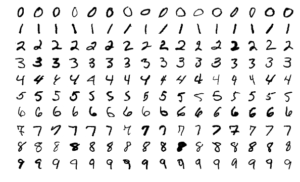
• A popular example of image classification is the MNIST (Modified National Institute of Standards and Technology) benchmark dataset for recognizing handwritten digits

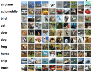
• CIFAR-10 and CIFAR-100 have photographs of various objects belonging to various classes

Why is image classification important?

In this data-driven world, we receive a huge amount of data from various devices, such as cameras and other IoT devices. Efficiently using these data can boost our productivity to a great extent.

We will see some of the applications of image classification that will establish the need for it:

• Object detection in self-driving cars
• Detecting tumors in an X-ray
• Face recognition

Image classification methods

Maximum likelihood and Minimum distance are two of the most common methods.

Image classification with TensorFlow

In this demo, we will build a simple image classifier using the sequential API of Keras and TensorFlow.

Before that, let us understand our dataset.

• It is an MNIST of handwritten digits.
• Each data point is a 2d array of 28*28 pixel
• It contains 60,000 training images and 10,000 testing images.
• It has 10 classes (0-9)
• It is the preliminary dataset; therefore, we often refer to it as hello world for ANN.

We will import the necessary libraries first –

import numpy as np

import matplotlib.pyplot as plt

import pandas as pd

import tensorflow as tf

import os

Now we will load the dataset:

mnist = tf.keras.datasets.mnist

(X_train_full, y_train_full), (X_test, y_test) = mnist.load_data()

After importing we can check the shape and data type of the imported dataset –

X_train_full.shape, X_train_full.dtype

Moving ahead we will normalize our dataset by dividing the pixels of features by 255 as the pixels range from 0 to 255 –

X_valid, X_train = X_train_full[: 5000] / 255., X_train_full[5000: ]/255.

y_valid, y_train = y_train_full[: 5000], y_train_full[5000:]

X_test = X_test/255.

Let us check how the image of our dataset looks:

plt.imshow(X_train[0], cmap=”binary”)

plt.axis(“off”)

plt.show()

y_train[0]

# cmap stands for the color map. Y_train[0] will tell us the label of the image.

# output

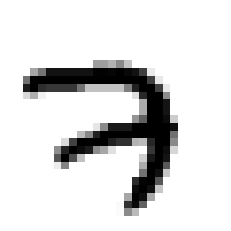
7

Let us check the same image using a heatmap for better clarity –

import seaborn as sns

plt.figure(figsize=(15,15))

sns.heatmap(X_train[0], annot=True, cmap=”binary”)

#output

We are done with pre-processing of the data. Now we will create layers of the ANN (Artificial Neural Network) model.

LAYERS = [

tf.keras.layers.Flatten(input_shape=[28, 28], name=”inputLayer”),

tf.keras.layers.Dense(300, activation=”relu”, name=”hiddenLayer1″),

tf.keras.layers.Dense(100, activation=”relu”, name=”hiddenLayer2″),

tf.keras.layers.Dense(10, activation=”softmax”, name=”outputLayer”),

]

# the first layer is the flattening, where we convert the two-dimensional array into a single dimension array of 784.

#in the following layer, 300,100,10 are the number of neurons present at each layer.

After creating the layers, we will now define the object of the model –

model = tf.keras.models.Sequential(LAYERS)

#Sequential means the layers are not skipped at any point in time.

Next, we can see the summary of the layers of the model –

model.summary()

#output

Model: “sequential_1”

_________________________________________________________________

Layer (type)                Output Shape              Param #

=================================================================

inputLayer (Flatten)        (None, 784)               0

hiddenLayer1 (Dense)        (None, 300)               235500

hiddenLayer2 (Dense)        (None, 100)               30100

outputLayer (Dense)         (None, 10)                1010

=================================================================

Total params: 266,610

Trainable params: 266,610

Non-trainable params: 0

Now that we are done arranging the layers of our model let us compile it now –

LOSS_FUNCTION = “sparse_categorical_crossentropy”

OPTIMIZER = “SGD”

METRICS = [“accuracy”]

model.compile(loss=LOSS_FUNCTION, optimizer=OPTIMIZER, metrics=METRICS)

After compiling our model, the obvious step is to train the model with the dataset we have loaded but before that, let us understand some key terminologies.

• Epochs: Integer.

An epoch is an iteration over the entire x and y data provided.

The user provides the number of epochs to train the model in integer format.

• batch_size: Integer or None.

The batch size provides the number of samples per gradient update. If unspecified, batch size will take a default value of 32.

NOTE: we do not specify the batch size if our data is in the form of datasets, generators, or keras.utils.Sequence instances (since they generate batches).

• validation_batch_size: Integer or None.

The number of samples per validation batch.

If left unspecified, it will take a default value equal to the batch_size.

NOTE: we do not specify the validation_batch_size if our data is in the form of datasets, generators, or keras.utils.Sequence instances (since they generate batches).

Now, let us train the model:

EPOCHS = 30

VALIDATION_SET = (X_valid, y_valid)

history = model.fit(X_train, y_train,epochs=EPOCHS,

validation_data=VALIDATION_SET)

#output will look something like this starting from 1/30 epochs –

Epoch 25/30

1719/1719 [==============================] – 4s 3ms/step – loss: 0.0237 – accuracy: 0.9951 – val_loss: 0.0673 – val_accuracy: 0.9790

Epoch 26/30

1719/1719 [==============================] – 4s 3ms/step – loss: 0.0226 – accuracy: 0.9954 – val_loss: 0.0673 – val_accuracy: 0.9786

Epoch 27/30

1719/1719 [==============================] – 4s 2ms/step – loss: 0.0213 – accuracy: 0.9958 – val_loss: 0.0676 – val_accuracy: 0.9778

Epoch 28/30

1719/1719 [==============================] – 4s 3ms/step – loss: 0.0202 – accuracy: 0.9962 – val_loss: 0.0678 – val_accuracy: 0.9794

Epoch 29/30

1719/1719 [==============================] – 4s 3ms/step – loss: 0.0193 – accuracy: 0.9966 – val_loss: 0.0670 – val_accuracy: 0.9800

Epoch 30/30

1719/1719 [==============================] – 4s 3ms/step – loss: 0.0182 – accuracy: 0.9969 – val_loss: 0.0671 – val_accuracy: 0.978

Training of the model is done, hence, we will now evaluate it –

model.evaluate(X_test, y_test)

#output

313/313 [==============================] – 1s 2ms/step – loss: 0.0678 – accuracy: 0.9793

[0.06781463325023651, 0.9793000221252441]

The output suggests an accuracy of 97.93% let’s check whether our model is able to predict it or not –

X_new = X_test[:3]

y_new = y_test[:3]

y_proba = model.predict(X_new)

y_proba.round(2)

#output

array([[0., 0., 0., 0., 0., 0., 0., 1., 0., 0.], [0., 0., 1., 0., 0., 0., 0., 0., 0., 0.], [0., 1., 0., 0., 0., 0., 0., 0., 0., 0.]], dtype=float32)

y_pred = np.argmax(y_proba, axis=-1)

y_pred, y_new

#output

(array([7, 2, 1]), array([7, 2, 1], dtype=uint8))

for data, pred, actual in zip(X_new, y_pred, y_new):

plt.imshow(data, cmap=”binary”)

plt.title(f”Predicted: {pred}, Actual: {actual}”)

plt.axis(“off”)

plt.show()

print(“—“*20)

#output

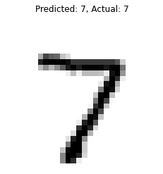
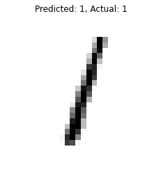
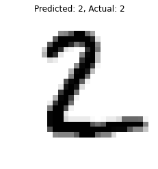
We can see that our model is giving correct predictions.

We can also save this model for future use using the following code –

model.save(“model.h5”) (#h5 is the name of the extension of the model)